# Loading our dataset
try:
from palmerpenguins import load_penguins
except:
! pip install palmerpenguins
from palmerpenguins import load_penguins
penguins = load_penguins()
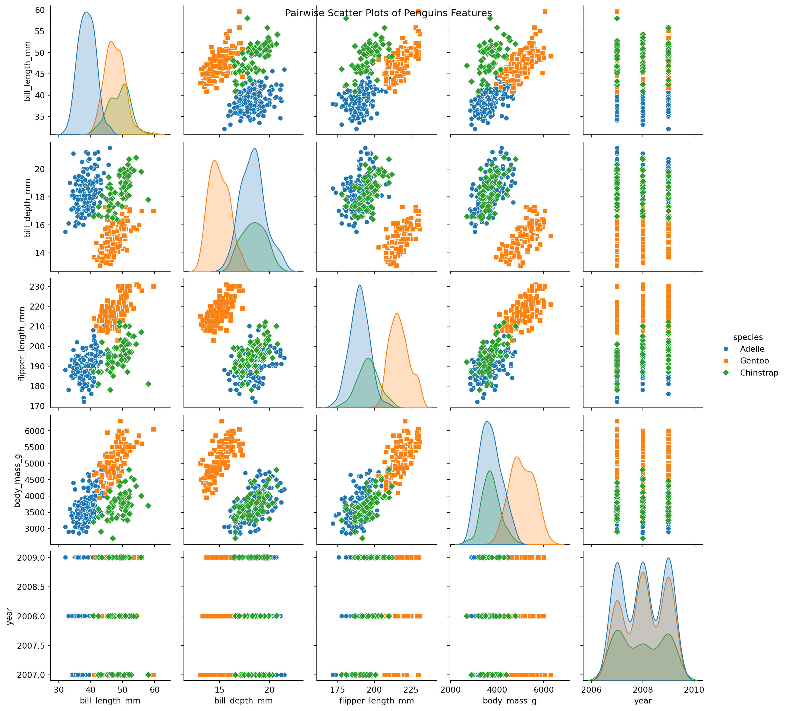
# Pairplot using seaborn
import matplotlib.pyplot as plt
import seaborn as sns
sns.pairplot(penguins, hue='species', markers=["o", "s", "D"])
plt.suptitle("Pairwise Scatter Plots of Penguins Features")
plt.show()Learning Algorithms
CSI 4106 - Fall 2025
Version: Sep 23, 2025 13:43
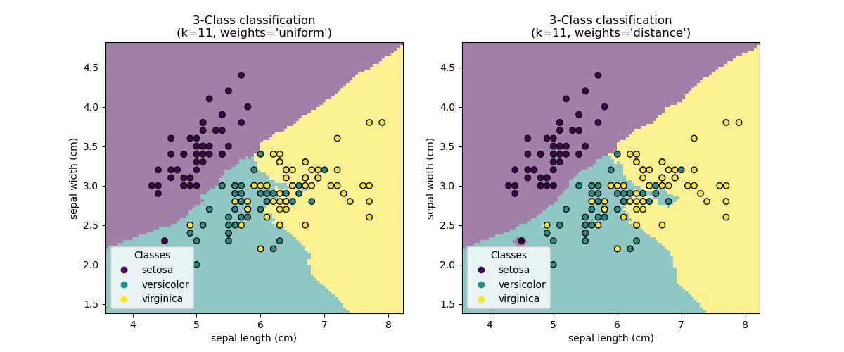
k-nearest neighbours (KNN)
Interpretable
Palmer Pinguins Dataset
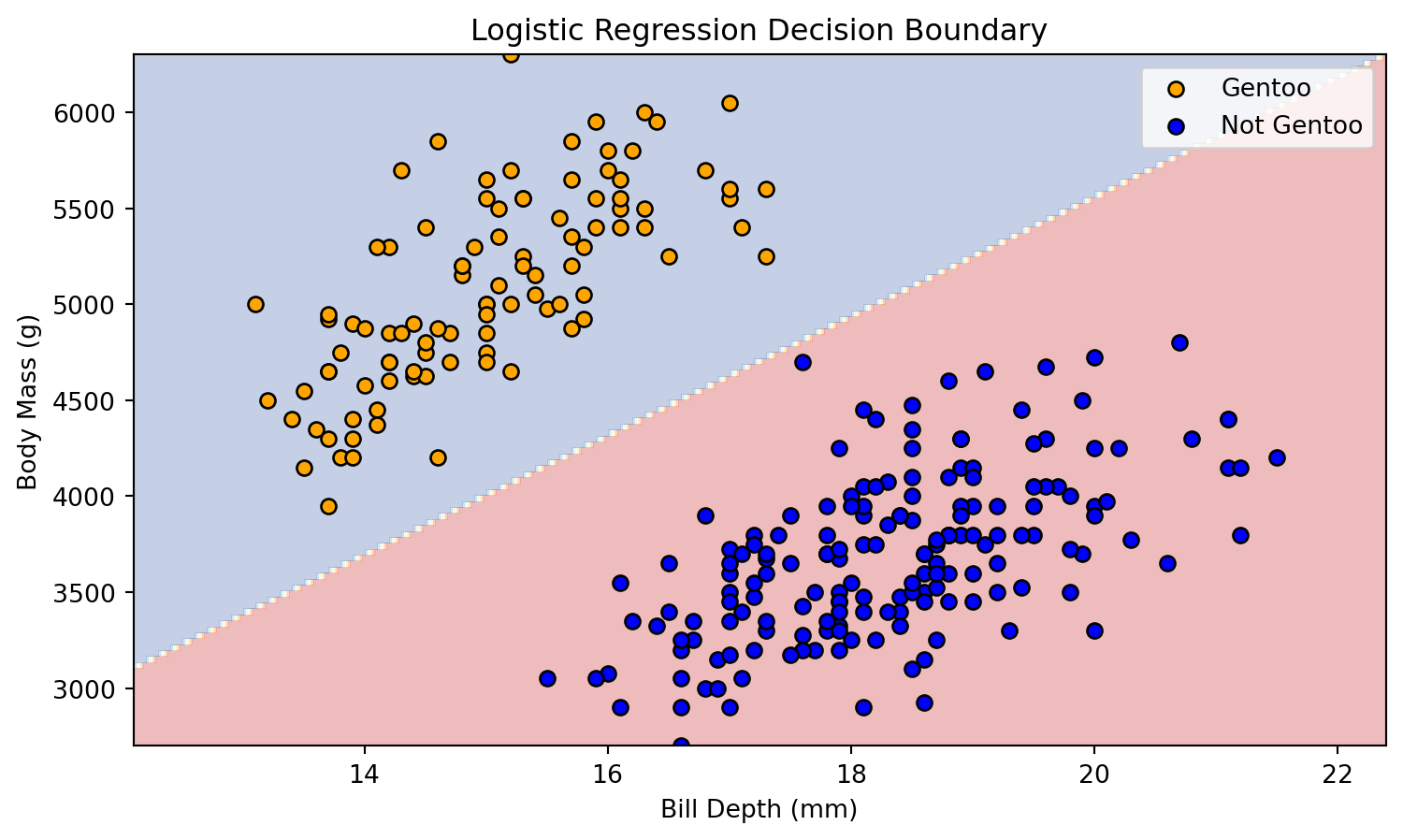
Decision Boundary
Decision Boundary
Simple Decision Doundary
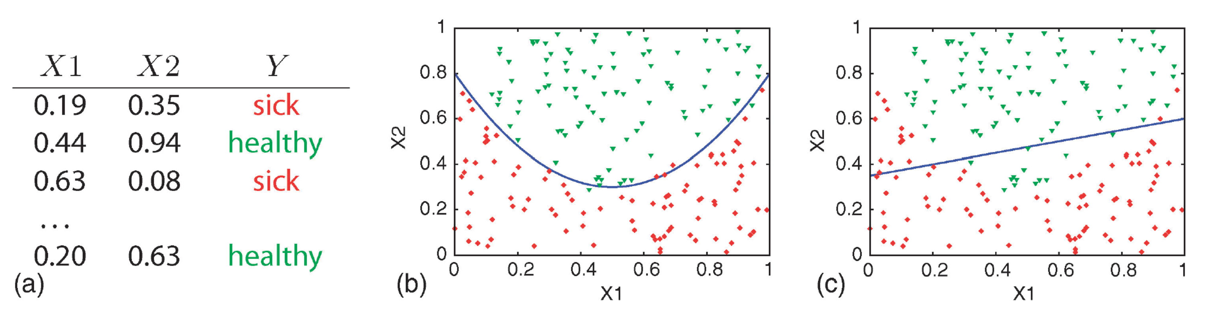
(a) training data, (b) quadratic curve, and (c) linear function.
Attribution: (Geurts, Irrthum, and Wehenkel 2009)
Complex Decision Boundary
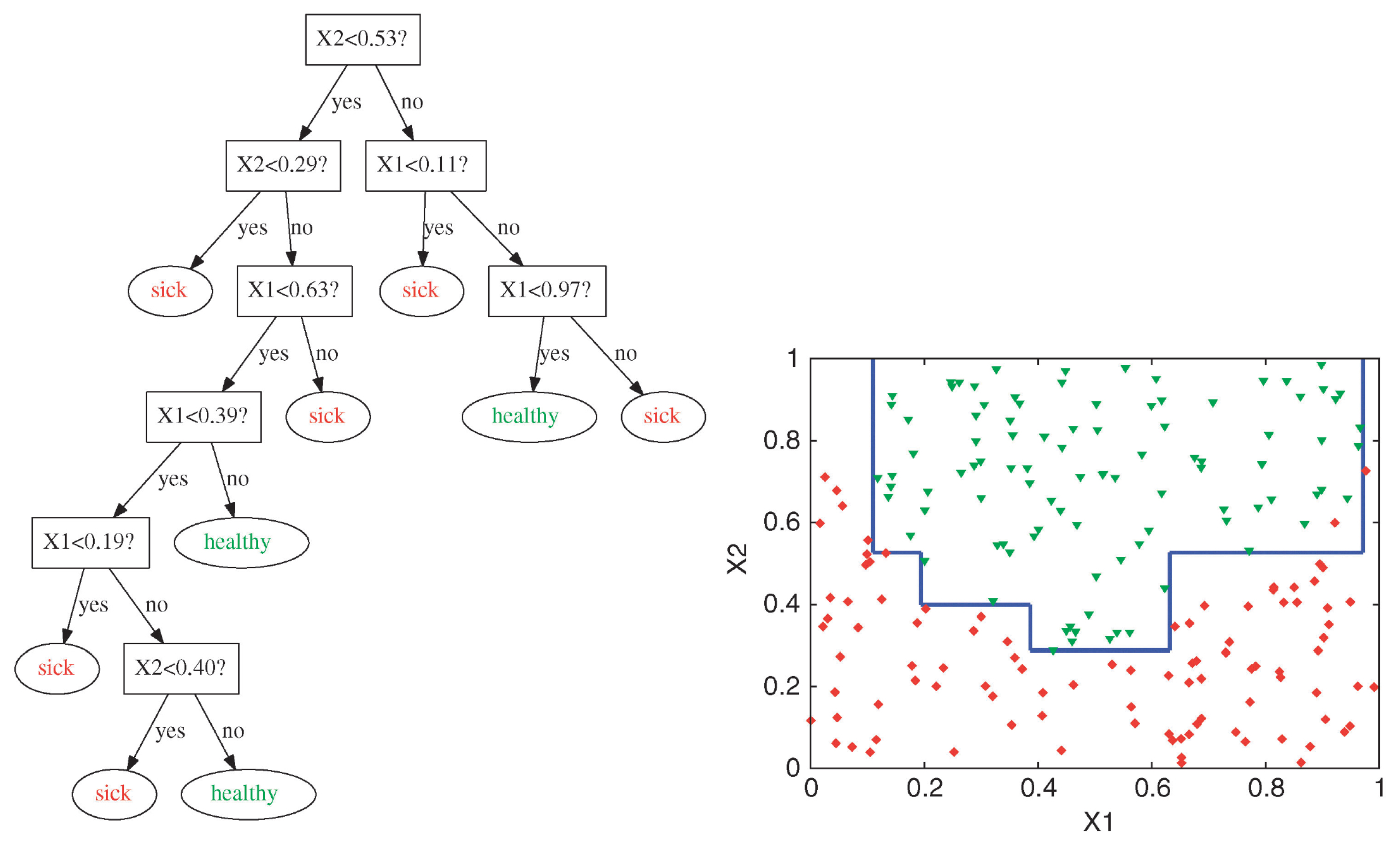
Decision trees are capable of generating irregular and non-linear decision boundaries.
Attribution: ibidem.
Gini Index
Code
def gini_index(p):
    """Calculate the Gini index."""
    return 1 - (p**2 + (1 - p)**2)

# Probability values for class 1
p_values = np.linspace(0, 1, 100)

# Calculate Gini index for each probability
gini_values = [gini_index(p) for p in p_values]

# Plot the Gini index
plt.figure(figsize=(8, 6))
plt.plot(p_values, gini_values, label='Gini Index', color='b')
plt.title('Gini Index for Binary Classification')
plt.xlabel('Probability of Class 1 (p)')
plt.ylabel('Gini Index')
plt.grid(True)
plt.legend()
plt.show()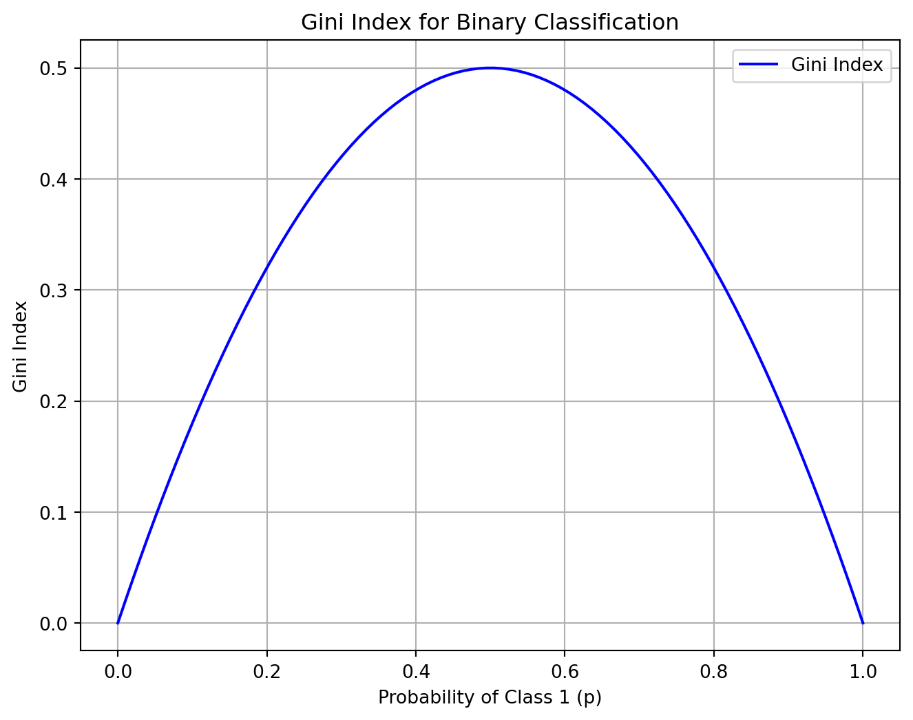
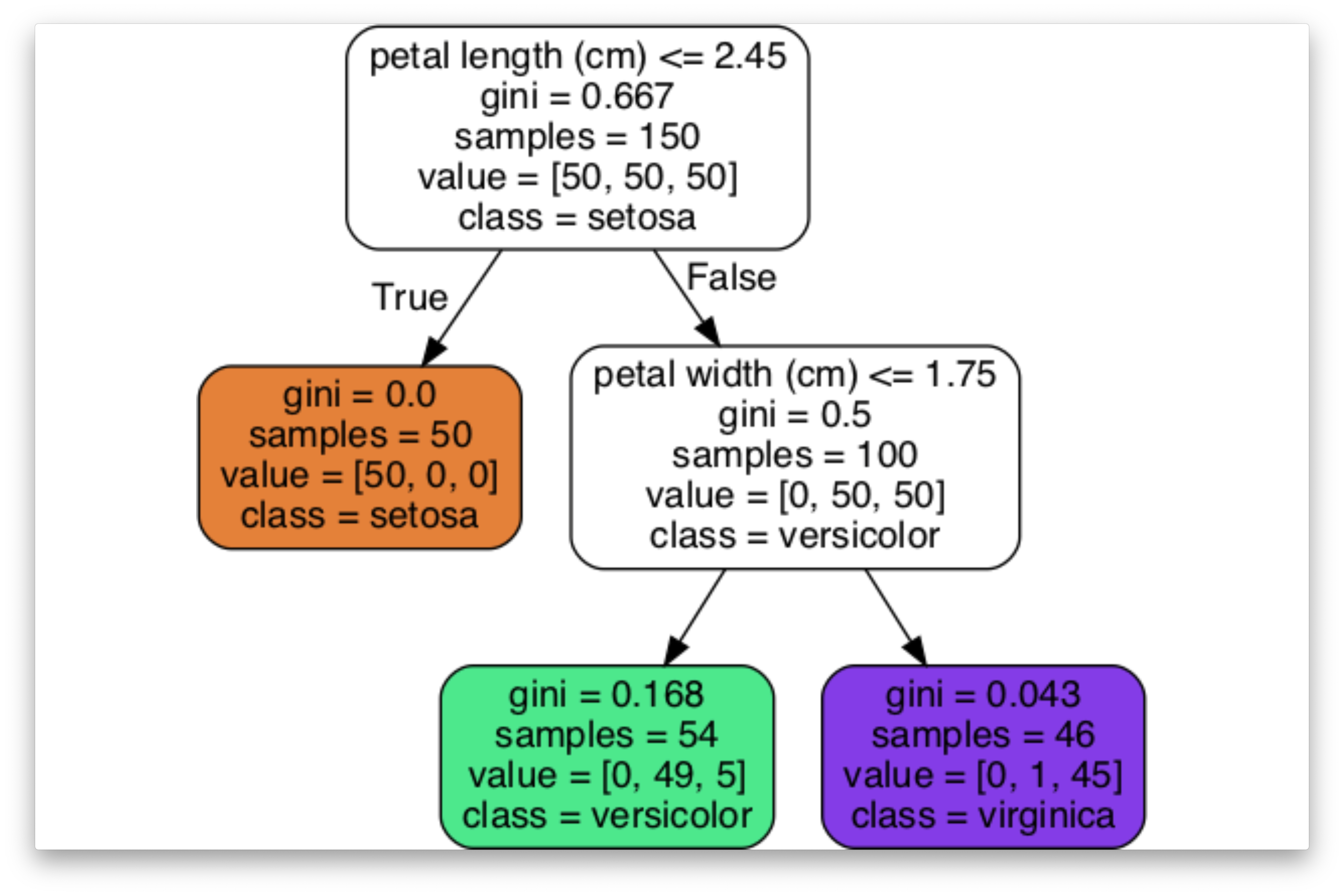
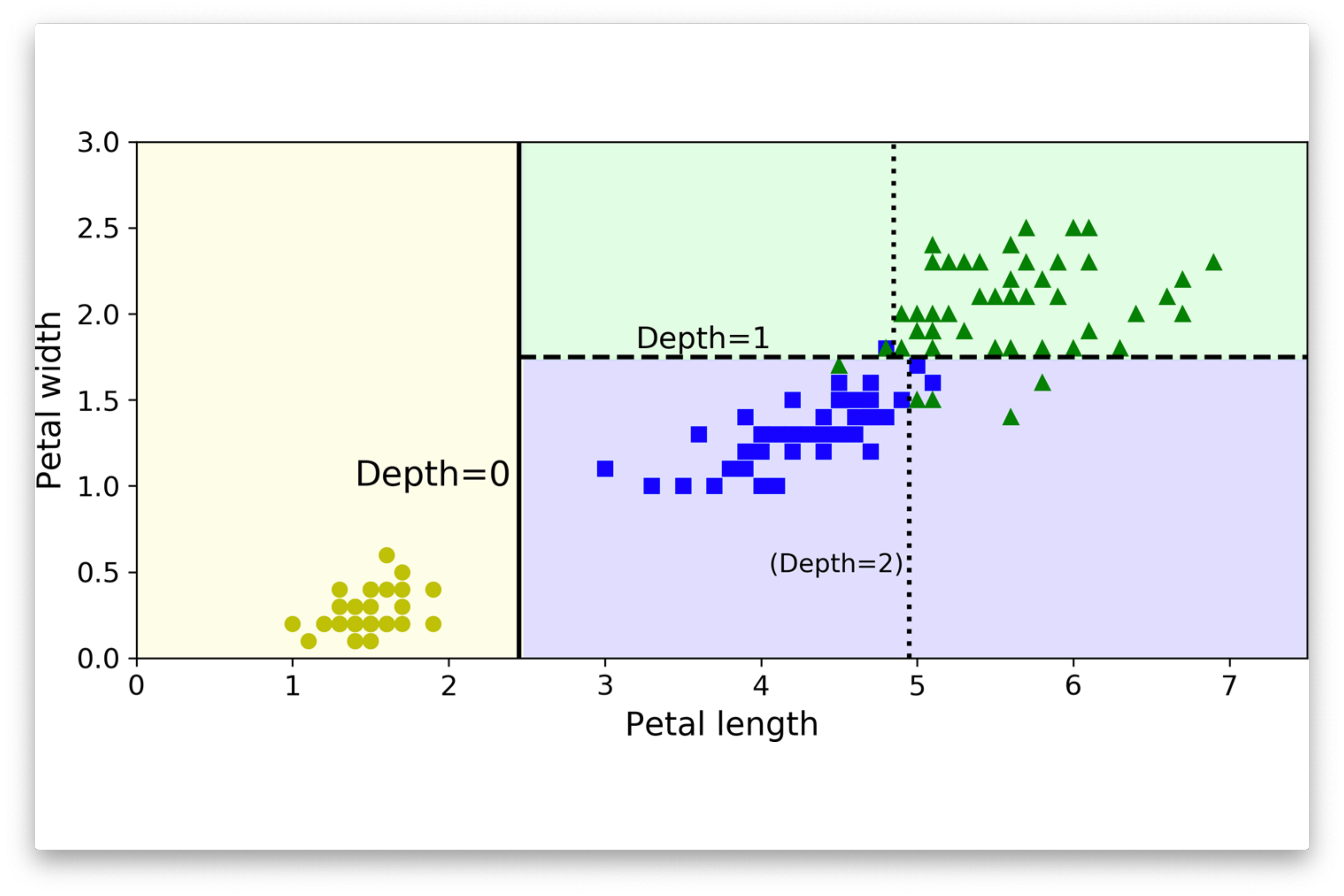
Iris Dataset
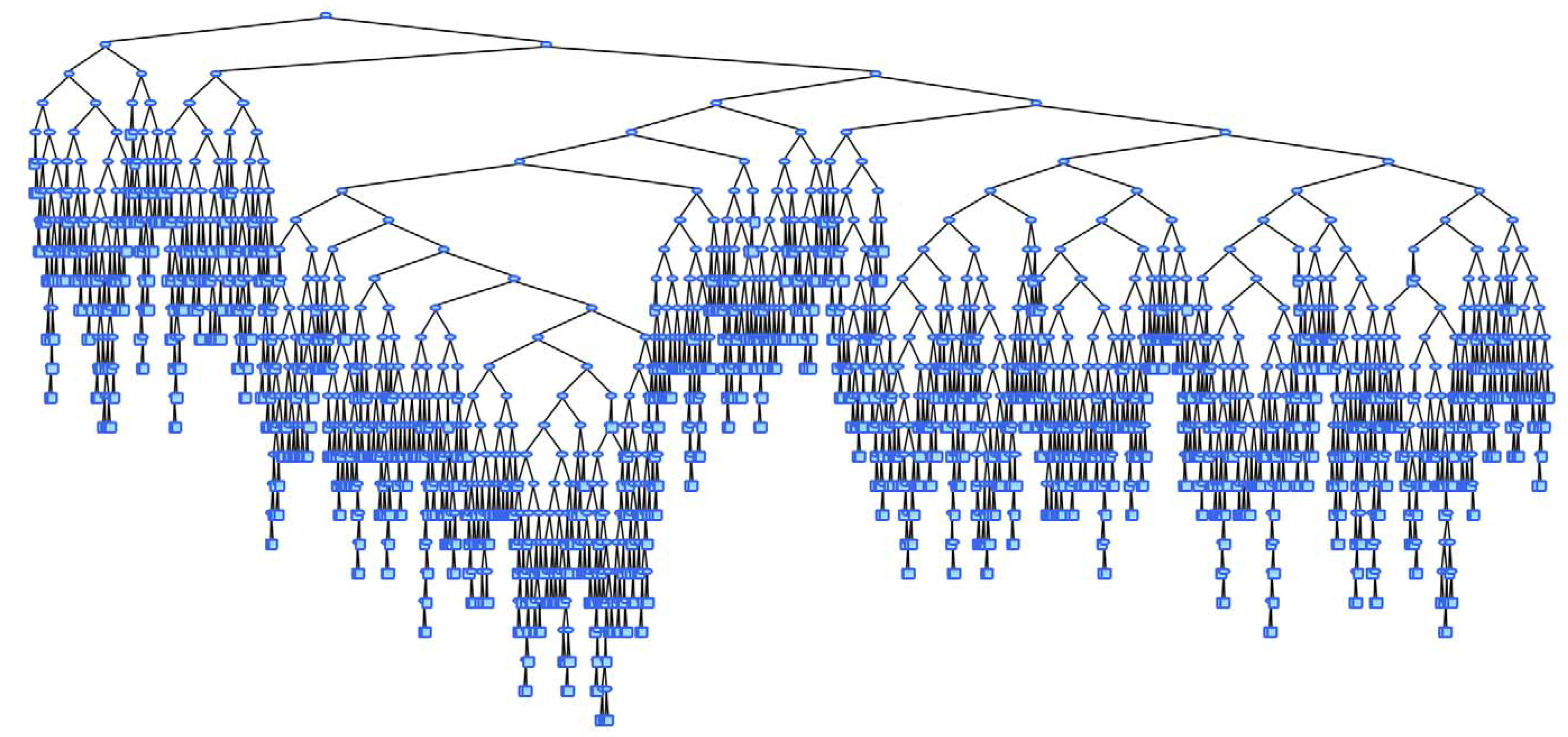
Large Trees
Small Changes to the Dataset
Seed: 4
Accuracy: 0.99
Classification Report:
              precision    recall  f1-score   support

      Adelie       1.00      0.97      0.99        36
   Chinstrap       0.94      1.00      0.97        17
      Gentoo       1.00      1.00      1.00        16

    accuracy                           0.99        69
   macro avg       0.98      0.99      0.99        69
weighted avg       0.99      0.99      0.99        69

Seed: 7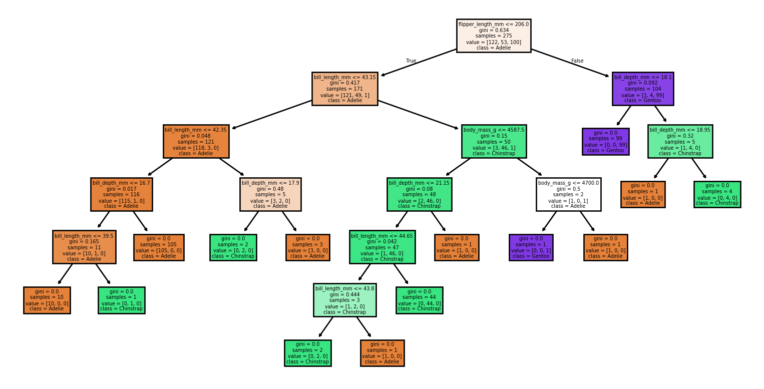
Accuracy: 0.91
Classification Report:
              precision    recall  f1-score   support

      Adelie       0.96      0.83      0.89        30
   Chinstrap       0.83      1.00      0.91        15
      Gentoo       0.92      0.96      0.94        24

    accuracy                           0.91        69
   macro avg       0.90      0.93      0.91        69
weighted avg       0.92      0.91      0.91        69

Seed: 90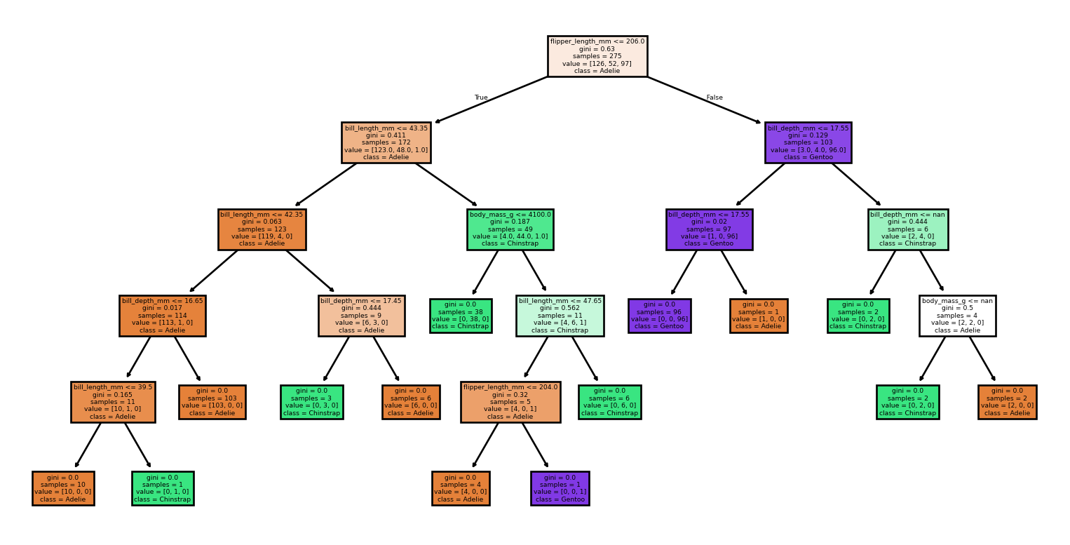
Accuracy: 0.94
Classification Report:
              precision    recall  f1-score   support

      Adelie       0.90      1.00      0.95        26
   Chinstrap       0.93      0.88      0.90        16
      Gentoo       1.00      0.93      0.96        27

    accuracy                           0.94        69
   macro avg       0.94      0.93      0.94        69
weighted avg       0.95      0.94      0.94        69

Seed: 96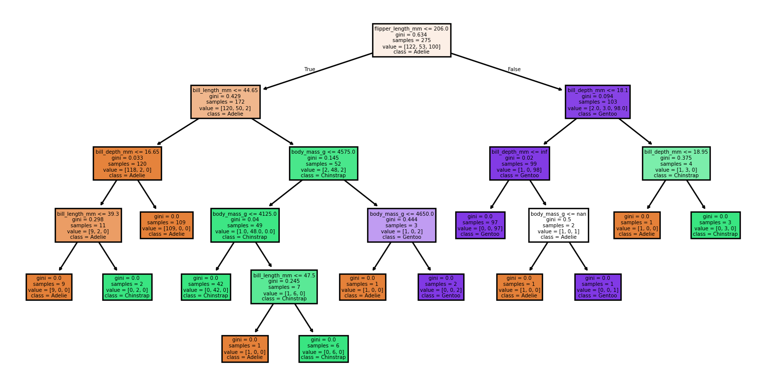
Accuracy: 0.90
Classification Report:
              precision    recall  f1-score   support

      Adelie       0.83      0.97      0.89        30
   Chinstrap       1.00      0.67      0.80        15
      Gentoo       0.96      0.96      0.96        24

    accuracy                           0.90        69
   macro avg       0.93      0.86      0.88        69
weighted avg       0.91      0.90      0.90        69

Seed: 99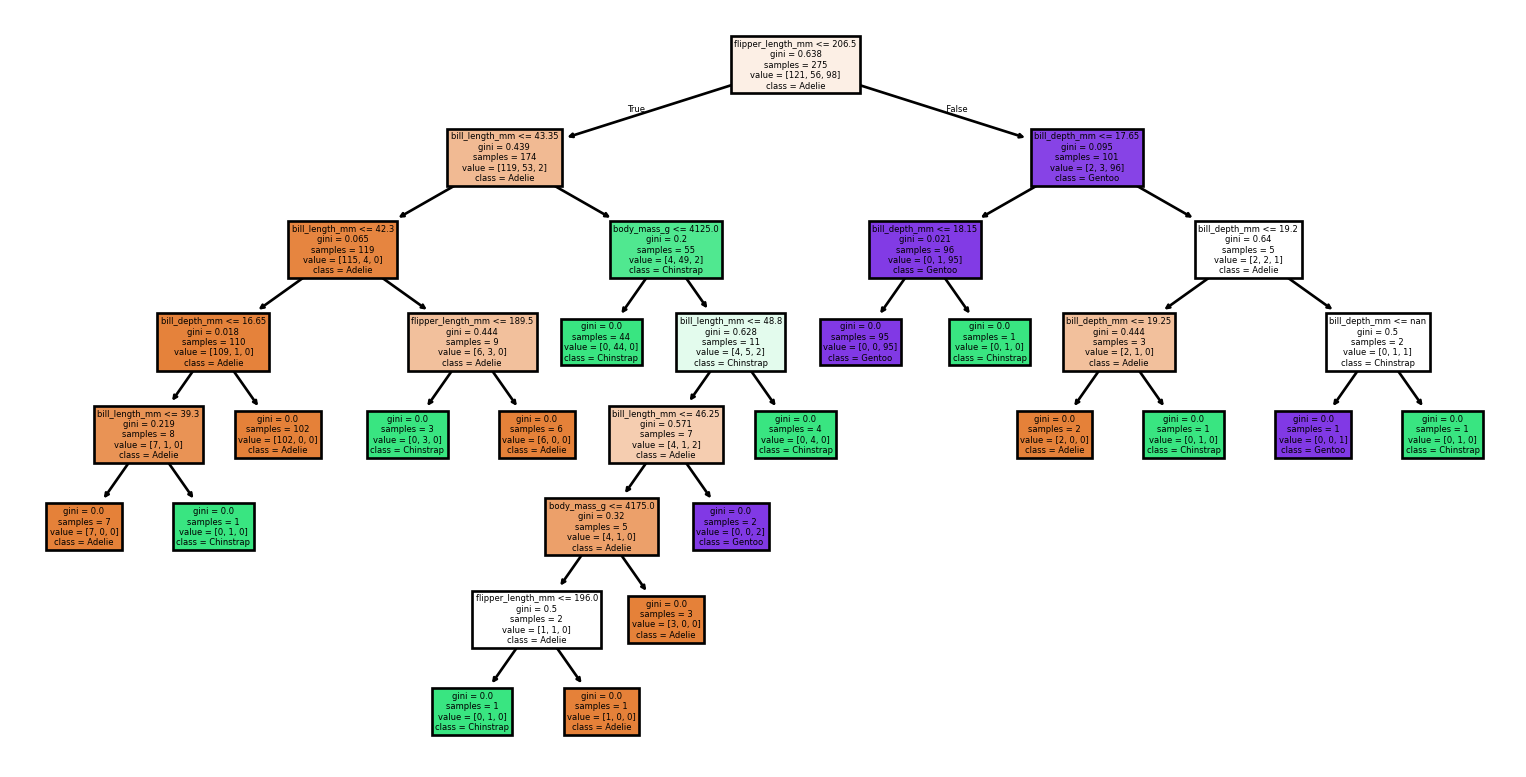
Accuracy: 1.00
Classification Report:
              precision    recall  f1-score   support

      Adelie       1.00      1.00      1.00        31
   Chinstrap       1.00      1.00      1.00        12
      Gentoo       1.00      1.00      1.00        26

    accuracy                           1.00        69
   macro avg       1.00      1.00      1.00        69
weighted avg       1.00      1.00      1.00        69

Seed: 2
Accuracy: 0.55
Classification Report:
              precision    recall  f1-score   support

      Adelie       0.62      0.97      0.75        30
   Chinstrap       0.43      0.90      0.58        10
      Gentoo       0.00      0.00      0.00        29

    accuracy                           0.55        69
   macro avg       0.35      0.62      0.44        69
weighted avg       0.33      0.55      0.41        69