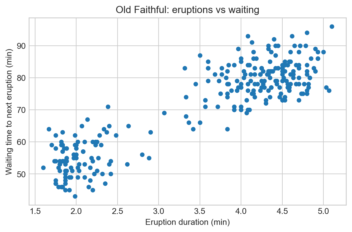
import pandas as pd

WOLFRAM_CSV = "https://raw.githubusercontent.com/turcotte/csi4106-f25/refs/heads/main/datasets/old_faithful_eruptions/Sample-Data-Old-Faithful-Eruptions.csv"
df = pd.read_csv(WOLFRAM_CSV)

# Renaming the columns
df = df.rename(columns={"Duration": "eruptions", "WaitingTime": "waiting"})
print(df.shape)
df.head(6)Linear regression and gradient descent
CSI 4106 - Fall 2025
Version: Sep 16, 2025 17:58
Message of the Day

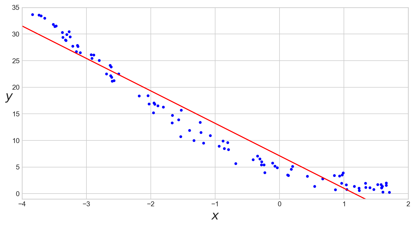
Quick Visualization

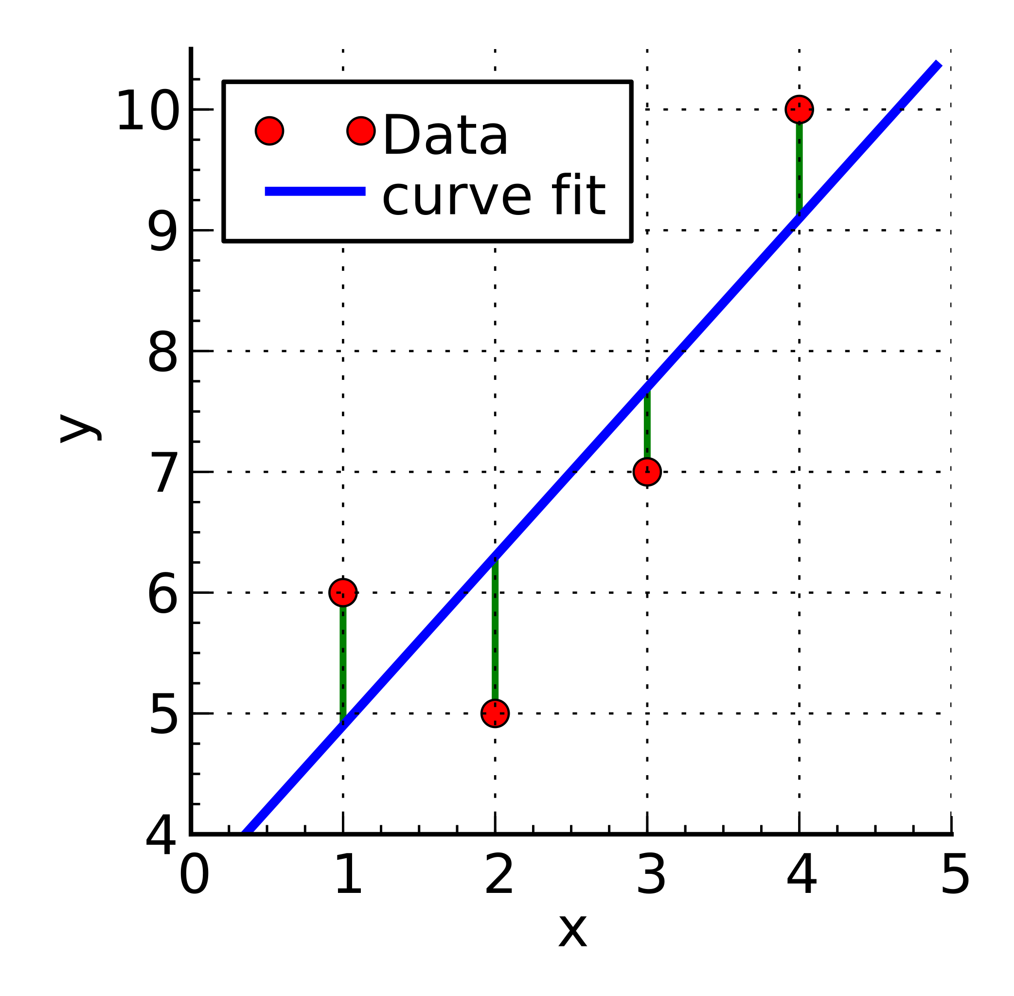
Minimizing RMSE
Visualization
Code
import numpy as np

# Scatter the data
plt.figure(figsize=(6,4))
plt.scatter(X, y, color="steelblue", s=30, alpha=0.7, label="data")

# Plot the fitted line
x_line = np.linspace(0, X.max(), 100).reshape(-1, 1)
y_line = sgd.predict(x_line)
plt.plot(x_line, y_line, color="red", linewidth=2, label="fitted line")

plt.xlabel("Eruption duration (min)")
plt.ylabel("Waiting time to next eruption (min)")
plt.title("Old Faithful: Linear regression via SGD")
plt.legend()
plt.tight_layout()
plt.show()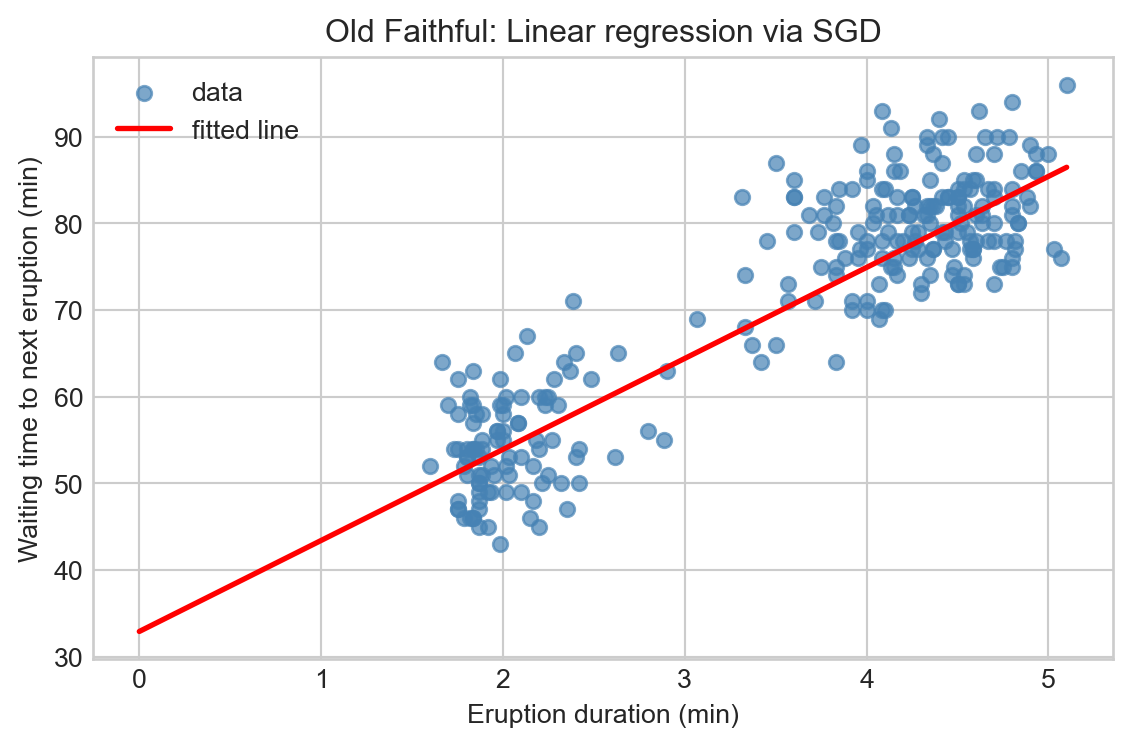
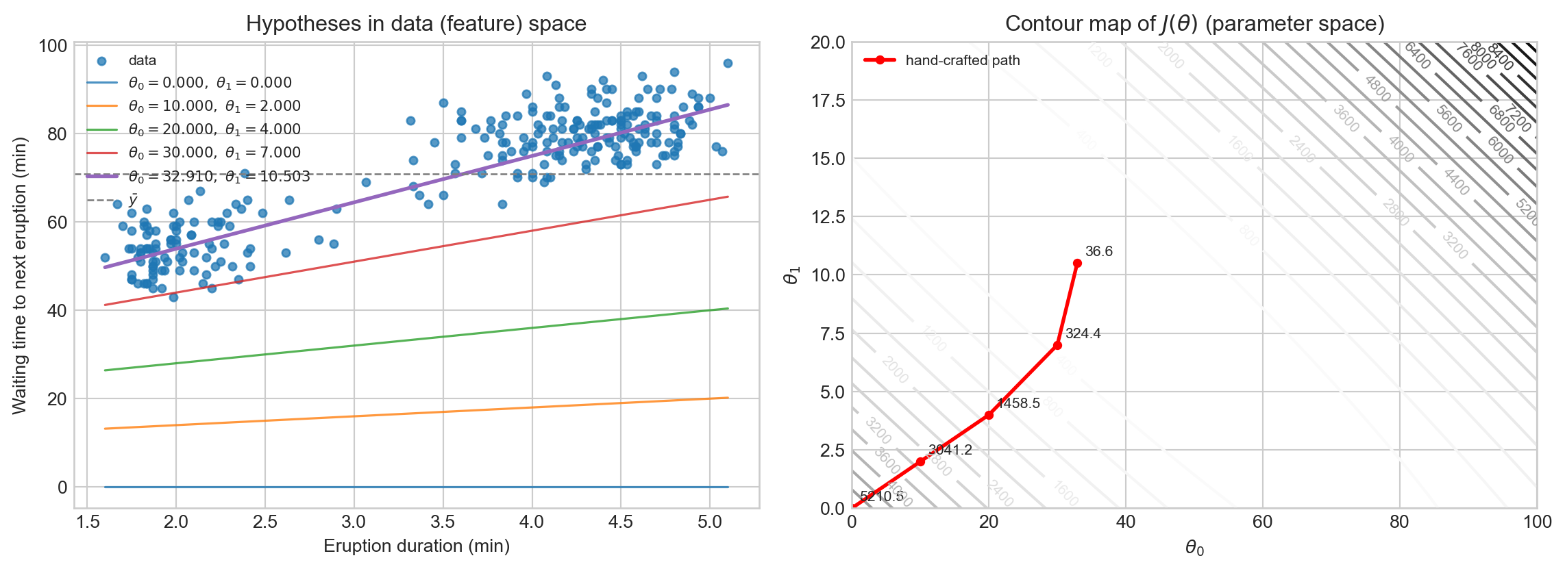
Hypothesis vs Parameter Space
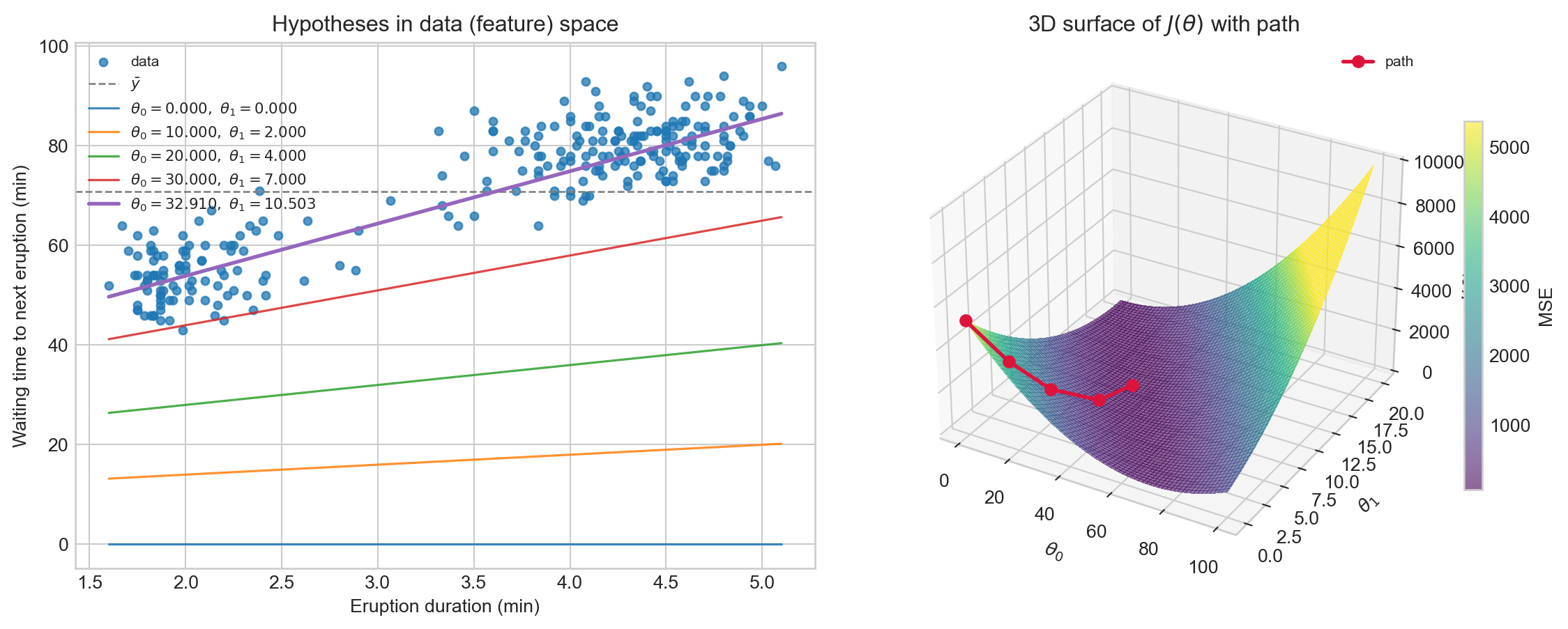
Hypothesis vs Parameter Space
Derivative

- We will start with a single-variable function.
- Think of this as our loss function, which we aim to minimize; to reduce the average discrepancy between expected and predicted values.
- Here, I am using \(t\) to avoid any confusion with the attributes of our training examples.
Derivative
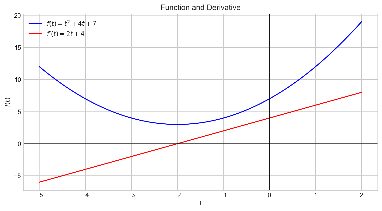
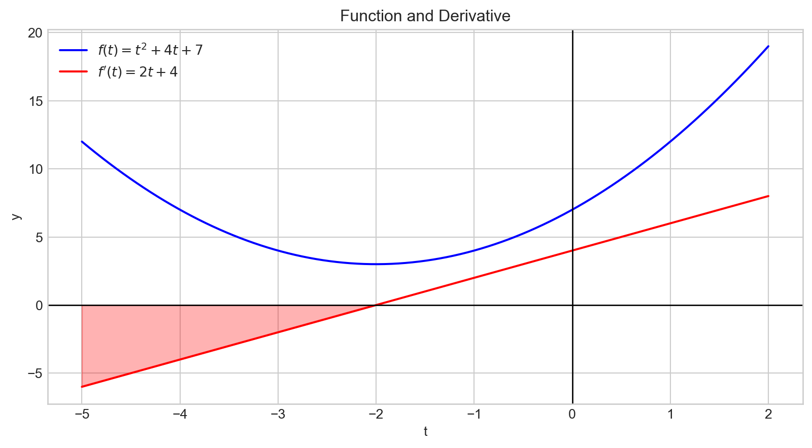
The graph of the derivative, \(f^{'}(t)\), is depicted in red.
The derivative indicates how changes in the input affect the output, \(f(t)\).
The magnitude of the derivative at \(t = -2\) is \(0\).
This point corresponds to the minimum of our function.
Derivative
- When evaluated at a specific point, the derivative indicates the slope of the tangent line to the graph of the function at that point.
- At \(t= -2\), the slope of the tangent line is 0.
Derivative
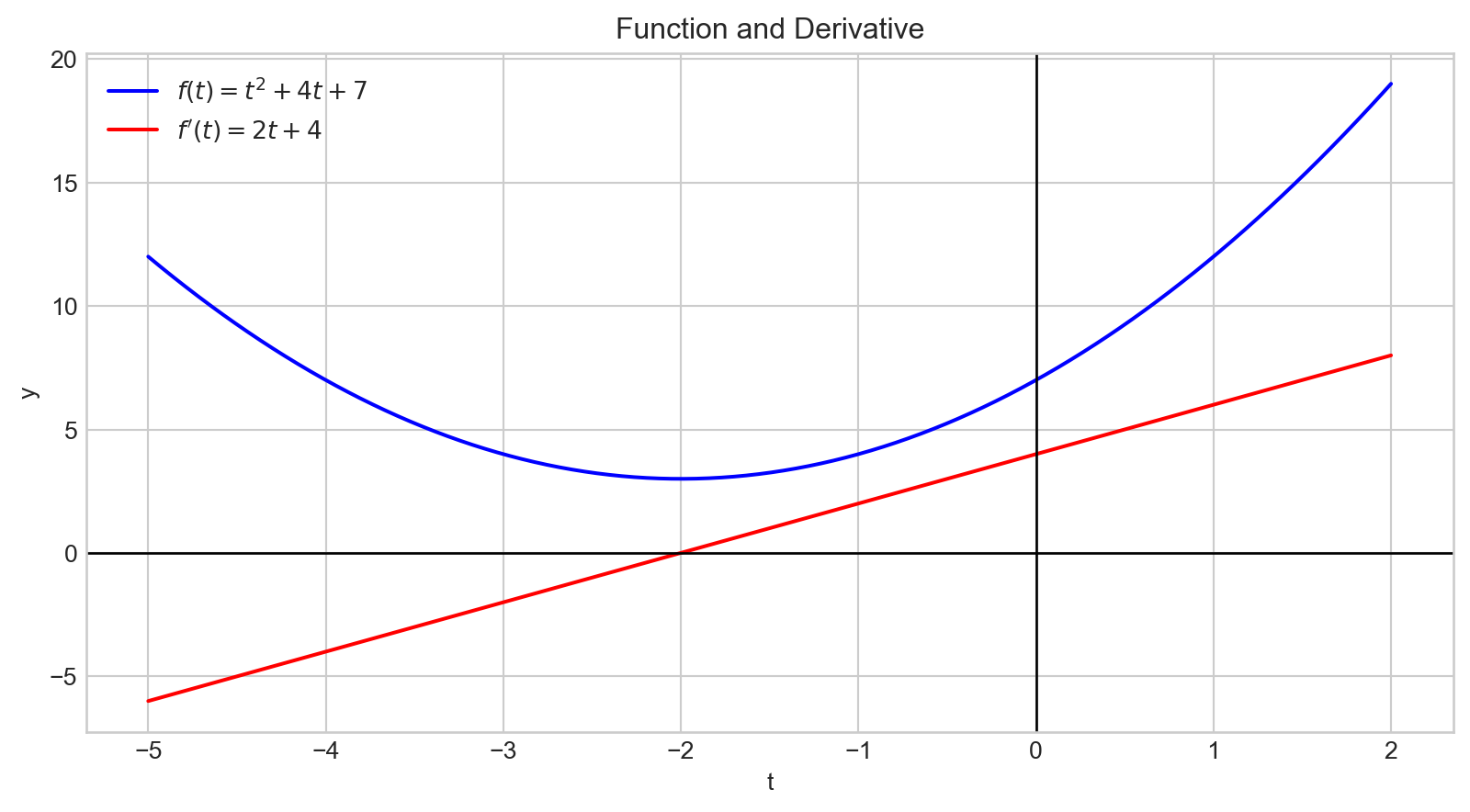
A positive derivative indicates that increasing the input variable will increase the output value.
Additionally, the magnitude of the derivative quantifies how rapidly the output changes.
Derivative
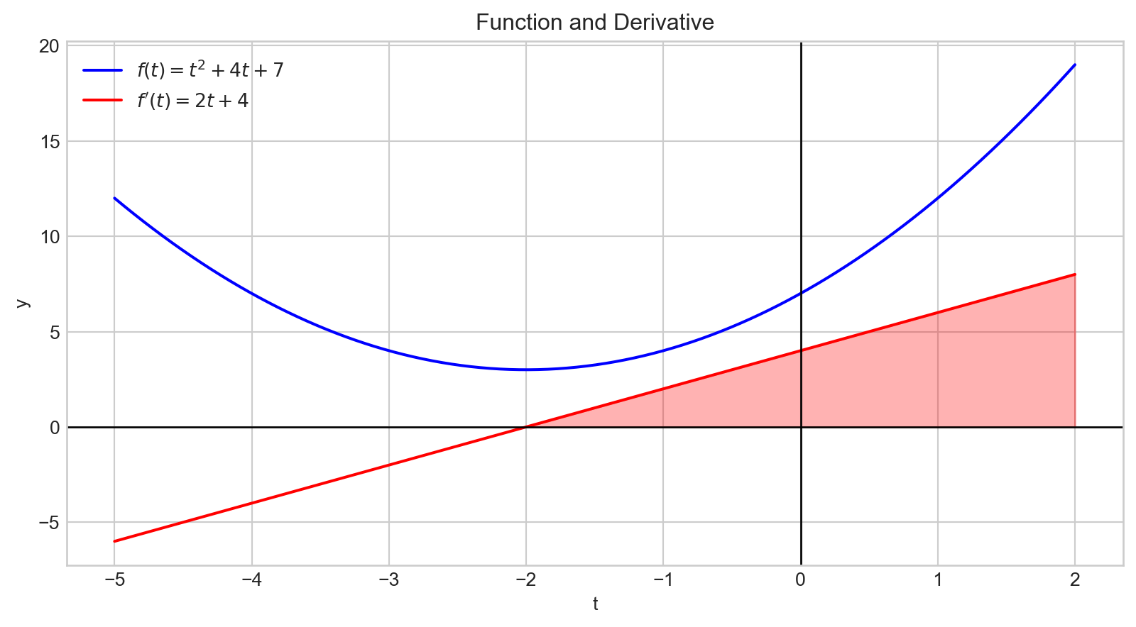
A negative derivative indicates that increasing the input variable will decrease the output value.
Additionally, the magnitude of the derivative quantifies how rapidly the output changes.
Gradient Descent - Single Value
Code
import sympy as sp
import numpy as np
import matplotlib.pyplot as plt

# Define the variable and function
t = sp.symbols('t')
f = t**2 + 4*t + 7

# Compute the derivative
f_prime = sp.diff(f, t)

# Lambdify the functions for numerical plotting
f_func = sp.lambdify(t, f, "numpy")
f_prime_func = sp.lambdify(t, f_prime, "numpy")

# Generate t values for plotting
t_vals = np.linspace(-5, 2, 400)

# Get y values for the function and its derivative
f_vals = f_func(t_vals)
f_prime_vals = f_prime_func(t_vals)

# Plot the function and its derivative
plt.plot(t_vals, f_vals, label=r'$J$', color='blue')
plt.plot(t_vals, f_prime_vals, label=r"$\frac {\partial}{\partial \theta_j}J(\theta)$", color='red')

# Add labels and legend
plt.axhline(0, color='black',linewidth=1)
plt.axvline(0, color='black',linewidth=1)
plt.title('Function and Derivative')
plt.xlabel(r'$\theta_j$')
plt.ylabel(r'$J$')
plt.legend()

# Show the plot
plt.grid(True)
plt.show()
When the value of \(\theta_j\) is in the range \([- \inf, -2)\), \(\frac {\partial}{\partial \theta_j}J(\theta)\) has a negative value.
Therefore, \(- \alpha \frac {\partial}{\partial \theta_j}J(\theta)\) is positive.
Accordingly, the value of \(\theta_j\) is increased.
Gradient Descent - Single Value
Code
import sympy as sp
import numpy as np
import matplotlib.pyplot as plt

# Define the variable and function
t = sp.symbols('t')
f = t**2 + 4*t + 7

# Compute the derivative
f_prime = sp.diff(f, t)

# Lambdify the functions for numerical plotting
f_func = sp.lambdify(t, f, "numpy")
f_prime_func = sp.lambdify(t, f_prime, "numpy")

# Generate t values for plotting
t_vals = np.linspace(-5, 2, 400)

# Get y values for the function and its derivative
f_vals = f_func(t_vals)
f_prime_vals = f_prime_func(t_vals)

# Plot the function and its derivative
plt.plot(t_vals, f_vals, label=r'$J$', color='blue')
plt.plot(t_vals, f_prime_vals, label=r"$\frac {\partial}{\partial \theta_j}J(\theta)$", color='red')

# Add labels and legend
plt.axhline(0, color='black',linewidth=1)
plt.axvline(0, color='black',linewidth=1)
plt.title('Function and Derivative')
plt.xlabel(r'$\theta_j$')
plt.ylabel(r'$J$')
plt.legend()

# Show the plot
plt.grid(True)
plt.show()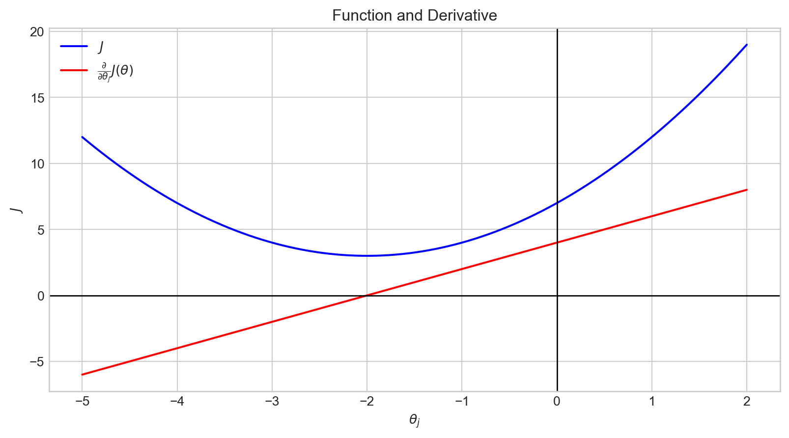
When the value of \(\theta_j\) is in the range \((-2, \infty]\), \(\frac {\partial}{\partial \theta_j}J(\theta)\) has a positive value.
Therefore, \(- \alpha \frac {\partial}{\partial \theta_j}J(\theta)\) is negative.
Accordingly, the value of \(\theta_j\) is decreased.
Local vs. global

Convergence
Code
# 1. Define the symbolic variable and the function
x = sp.Symbol('x', real=True)
f_expr = 2*x**3 + 4*x**2 - 5*x + 1

# 2. Compute the derivative of f
f_prime_expr = sp.diff(f_expr, x)

# 3. Convert symbolic expressions to Python functions
f = sp.lambdify(x, f_expr, 'numpy')
f_prime = sp.lambdify(x, f_prime_expr, 'numpy')

# 4. Generate a range of x-values
x_vals = np.linspace(-4, 2, 1000)

# 5. Compute f and f' over this range
y_vals = f(x_vals)
y_prime_vals = f_prime(x_vals)

# 6. Prepare LaTeX strings for legend
f_label = rf'$f(x) = {sp.latex(f_expr)}$'
f_prime_label = rf'$f^\prime(x) = {sp.latex(f_prime_expr)}$'

# 7. Plot f and f', with equations in the legend
plt.figure(figsize=(8, 4))
plt.plot(x_vals, y_vals, label=f_label)
plt.plot(x_vals, y_prime_vals, label=f_prime_label)

# 8. Shade the region between x-axis and f'(x) for the entire domain
plt.fill_between(x_vals, y_prime_vals, 0, color='gray', alpha=0.2, interpolate=True,
                 label='Region between 0 and f\'(x)')

# 9. Add reference line, labels, legend, etc.
plt.axhline(0, color='black', linewidth=0.5)
plt.title(rf'Function and its Derivative with Shading for $f^\prime(x)$')
plt.xlabel('x')
plt.ylabel('y')
plt.legend()
plt.grid(True)
plt.show()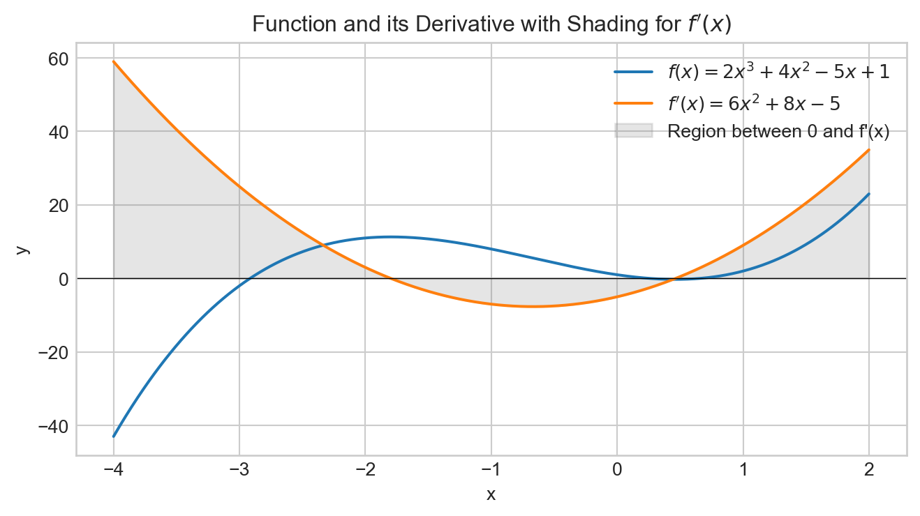
Learning Rate
- Small steps, low values for \(\alpha\), will make the algorithm converge slowly.
- Large steps might cause the algorithm to diverge.
- Notice how the algorithm slows down naturally when approaching a minimum.
Learning Rate
Code
import numpy as np
import matplotlib.pyplot as plt

def f(x):
    return x**2

def grad_f(x):
    return 2*x

# Initial guess, learning rate, and number of gradient-descent steps
x_current = 2.0
learning_rate = 1.1  # Too large => divergence
num_iterations = 5   # We'll do five updates

# Store each x value in a list (trajectory) for plotting
trajectory = [x_current]

# Perform gradient descent
for _ in range(num_iterations):
    g = grad_f(x_current)
    x_current = x_current - learning_rate * g
    trajectory.append(x_current)

# Prepare data for plotting
x_vals = np.linspace(-5, 5, 1000)
y_vals = f(x_vals)

# Plot the function f(x)
plt.figure(figsize=(6, 5))
plt.plot(x_vals, y_vals, label=r"$f(x) = x^2$")
plt.axhline(0, color='black', linewidth=0.5)

# Plot the trajectory, labeling each iteration
for i, x_t in enumerate(trajectory):
    y_t = f(x_t)
    # Plot the point
    plt.plot(x_t, y_t, 'ro')
    # Label the iteration number
    plt.text(x_t, y_t, f"  {i}", color='red')
    # Connect consecutive points
    if i > 0:
        x_prev = trajectory[i - 1]
        y_prev = f(x_prev)
        plt.plot([x_prev, x_t], [y_prev, y_t], 'r--')

# Final touches
plt.title("Gradient Descent Divergence with a Large Learning Rate")
plt.xlabel("x")
plt.ylabel("f(x)")
plt.legend()
plt.grid(True)
plt.show()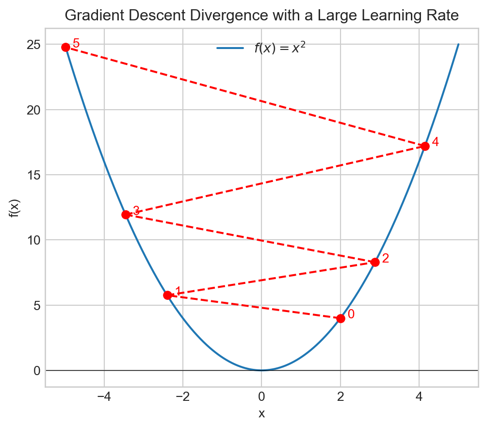
Quick Visualization
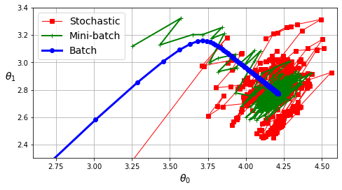
Stochastic, Mini-Batch, Batch
Andrew Ng
- Gradient Descent (Math)
(11:30 m) - Intuition
(11:51 m) - Linear Regression
(10:20 m) - ML-005 | Stanford | Andrew Ng
(19 videos)
LinearRegression