Cross-entropy, geometric interpretation, and implementation

CSI 4106 - Fall 2025

Marcel Turcotte

Version: Sep 16, 2025 17:17

Preamble

Message of the Day

TIME conducted interviews with the authors of a recent report from the Stanford Digital Economy Lab, titled “Canaries in the Coal Mine? Six Facts about the Recent Employment Effects of Artificial Intelligence.” The report is available here and here is the abstract:

This paper examines changes in the labor market for occupations exposed to generative artificial intelligence using high-frequency administrative data from the largest payroll software provider in the United States. We present six facts that characterize these shifts. We find that since the widespread adoption of generative AI, early-career workers (ages 22-25) in the most AI-exposed occupations have experienced a 13 percent relative decline in employment even after controlling for firm-level shocks. In contrast, employment for workers in less exposed fields and more experienced workers in the same occupations has remained stable or continued to grow. We also find that adjustments occur primarily through employment rather than compensation. Furthermore, employment declines are concentrated in occupations where AI is more likely to automate, ratherthanaugment, humanlabor. Ourresultsarerobusttoalternativeexplanations, such as excluding technology-related firms and excluding occupations amenable to remote work. These six facts provide early, large-scale evidence consistent with the hypothesis that the AI revolution is beginning to have a significant and disproportionate impact on entry-level workers in the American labor market.

AI’s “Significant Effect” on Entry-Level Work, TIME, 2025-09-05. (13m 55s)

Learning Outcomes

By the end of this presentation, you should be able to:

• Differentiate between MSE and cross-entropy as loss functions.
• Relate maximum likelihood estimation to parameter learning in logistic regression.
• Interpret the geometric view of logistic regression as a linear decision boundary.
• Implement logistic regression with gradient descent on simple data.

Linear Regression

Problem

• General Case: \(P(y = k \mid x, \theta)\), where \(k\) is a class label.
• Binary Case: \(y \in {0,1}\)
  • Predict \(P(y = 1 \mid x, \theta)\)

For a new instance \(x_{\textrm{new}}\), determine the probability that it belongs to class \(k\), denoted as \(P(y = k \mid x_{\textrm{new}}, \theta)\).

Logistic Regression

The Logistic Regression model is defined as:

\[ h_\theta(x_i) = \sigma(\theta x_i) = \frac{1}{1+e^{- \theta x_i}} \]

• Predictions are made as follows:

• \(y_i = 0\), if \(h_\theta(x_i) < 0.5\)

• \(y_i = 1\), if \(h_\theta(x_i) \geq 0.5\)

In the previous lecture, we considered an example wherein logistic regression was used to classify handwritten digits.

• The classification problem was addressed using a one-vs-rest strategy, which involved training ten separate logistic regression models, each dedicated to recognizing a specific digit.
• Each model consisted of 65 parameters: one bias term and 64 weights. Each weight corresponded to a pixel (or attribute) of a \(64 \times 64\) pixel image.
• This method demonstrated an excellent performance, achieving an overall accuracy of 0.97.
• Analyzing the weights provided insights into the areas of the image to which the model was most responsive (what does it pay attention to?).

The model presented above is expressed in its vectorized form, allowing it to be applied to problems involving multiple attributes. In the context of recognizing handwritten digits, the model utilizes 64 attributes, corresponding to individual pixels. The function \(\sigma\) employed in this model is the logistic, or sigmoid, function.

The problem is formulated as a binary classification task, wherein the model presumes that the classes are separable by a linear function within the feature space.

Loss Function

Model Overview

• Our model is expressed in a vectorized form as:

  \[ h_\theta(x_i) = \sigma(\theta x_i) = \frac{1}{1+e^{- \theta x_i}} \]

• Prediction:

  • Assign \(y_i = 0\), if \(h_\theta(x_i) < 0.5\); \(y_i = 1\), if \(h_\theta(x_i) \geq 0.5\)

• The parameter vector \(\theta\) is optimized using gradient descent.

• Which loss function should be used and why?

In logistic regression, the output is regarded as a probability, with particular emphasis on the interpretation process.

Remarks

• In constructing machine learning models with libraries like scikit-learn or keras, one has to select a loss function or accept the default one.

• Initially, the terminology can be confusing, as identical functions may be referenced by various names.

• Our aim is to elucidate these complexities.

• It is actually not that complicated!

Parameter Estimation

• Logistic regression is statistical model.

• Its output is \(\hat{y} = P(y = 1 | x, \theta)\).

• \(P(y = 0 | x, \theta) = 1 - \hat{y}\).

• Assumes that \(y\) values come from a Bernoulli distribution.

• \(\theta\) is commonly found by Maximum Likelihood Estimation.

The expressions \(\hat{y}\), \(h_\theta(x_i)\), and \(\sigma(\theta x_i)\) represent the same concept, albeit at varying levels of abstraction and specificity.

Parameter Estimation

Maximum Likelihood Estimation (MLE) is a statistical method used to estimate the parameters of a probabilistic model.

It identifies the parameter values that maximize the likelihood function, which measures how well the model explains the observed data.

Likelihood Function

Assuming the \(y\) values are independent and identically distributed (i.i.d.), the likelihood function is expressed as the product of individual probabilities.

In other words, given our data, \(\{(x_i, y_i)\}_{i=1}^N\), the likelihood function is given by this equation. \[ \mathcal{L}(\theta) = \prod_{i=1}^{N} P(y_i \mid x_i, \theta) \]

Maximum Likelihood

\[ \hat{\theta} = \underset{\theta \in \Theta}{\arg \max} \mathcal{L}(\theta) = \underset{\theta \in \Theta}{\arg \max} \prod_{i=1}^{N} P(y_i \mid x_i, \theta) \]

• Observations:

  1. Maximizing a function is equivalent to minimizing its negative.
  2. The logarithm of a product equals the sum of its logarithms.

Negative Log-Likelihood

Maximum likelihood \[ \hat{\theta} = \underset{\theta \in \Theta}{\arg \max} \mathcal{L}(\theta) = \underset{\theta \in \Theta}{\arg \max} \prod_{i=1}^{N} P(y_i \mid x_i, \theta) \]

becomes negative log-likelihood

\[ \hat{\theta} = \underset{\theta \in \Theta}{\arg \min} - \log \mathcal{L(\theta)} = \underset{\theta \in \Theta}{\arg \min} - \log \prod_{i=1}^{N} P(y_i \mid x_i, \theta) = \underset{\theta \in \Theta}{\arg \min} - \sum_{i=1}^{N} \log P(y_i \mid x_i, \theta) \]

Mathematical Reformulation

For binary outcomes, the probability \(P(y \mid x, \theta)\) is:

\[ P(y \mid x, \theta) = \begin{cases} \sigma(\theta x), & \text{if}\ y = 1 \\ 1 - \sigma(\theta x), & \text{if}\ y = 0 \end{cases} \]

This can be compactly expressed as:

\[ P(y \mid x, \theta) = \sigma(\theta x)^y (1 - \sigma(\theta x))^{1-y} \]

This “mathematical hack” validates the rationale for the label encoding.

Loss Function

We are now ready to write our loss function.

\[ J(\theta) = - \log \mathcal{L(\theta)} = - \sum_{i=1}^{N} \log P(y_i \mid x_i, \theta) \] where \(P(y \mid x, \theta) = \sigma(\theta x)^y (1 - \sigma(\theta x))^{1-y}\).

Consequently, \[ J(\theta) = - \sum_{i=1}^{N} \log [ \sigma(\theta x_i)^{y_i} (1 - \sigma(\theta x_i))^{1-y_i} ] \]

Loss Function (continued)

Simplifying the equation. \[ J(\theta) = - \sum_{i=1}^{N} \log [ \sigma(\theta x_i)^{y_i} (1 - \sigma(\theta x_i))^{1-y_i} ] \] by distributing the \(\log\) into the square parenthesis. \[ J(\theta) = - \sum_{i=1}^{N} [ \log \sigma(\theta x_i)^{y_i} + \log (1 - \sigma(\theta x_i))^{1-y_i} ] \]

Loss Function (continued)

Simplifying the equation further. \[ J(\theta) = - \sum_{i=1}^{N} [ \log \sigma(\theta x_i)^{y_i} + \log (1 - \sigma(\theta x_i))^{1-y_i} ] \] by moving the exponents in front of the \(\log\)s.

\[ J(\theta) = - \sum_{i=1}^{N} [ y_i \log \sigma(\theta x_i) + (1-y_i) \log (1 - \sigma(\theta x_i)) ] \]

The rationale for these additional simplifications will be elucidated shortly.

One More Thing

• Decision tree algorithms often employ entropy, a measure from information theory, to evaluate the quality of splits or partitions in decision rules.
• Entropy quantifies the uncertainty or impurity associated with the potential outcomes of a random variable.

Entropy

Entropy in information theory quantifies the uncertainty or unpredictability of a random variable’s possible outcomes. It measures the average amount of information produced by a stochastic source of data and is typically expressed in bits for binary systems. The entropy \(H\) of a discrete random variable \(X\) with possible outcomes \(\{x_1, x_2, \ldots, x_n\}\) and probability mass function \(P(X)\) is given by:

\[ H(X) = -\sum_{i=1}^n P(x_i) \log_2 P(x_i) \]

Cross-Entropy

Cross-entropy quantifies the difference between two probability distributions, typically the true distribution and a predicted distribution.

\[ H(p, q) = -\sum_{i} p(x_i) \log q(x_i) \] where \(p(x_i)\) is the true probability distribution, and \(q(x_i)\) is the predicted probability distribution.

Cross-Entropy

• Consider \(y\) as the true probability distribution and \(\hat{y}\) as the predicted probability distribution.
• Cross-entropy quantifies the discrepancy between these two distributions.

Cross-Entropy

Consider the negative log-likelihood loss function:

\[ J(\theta) = - \sum_{i=1}^{N} \left[ y_i \log \sigma(\theta x_i) + (1-y_i) \log (1 - \sigma(\theta x_i)) \right] \]

By substituting \(\sigma(\theta x_i)\) with \(\hat{y_i}\), the function becomes:

\[ J(\theta) = - \sum_{i=1}^{N} \left[ y_i \log \hat{y_i} + (1-y_i) \log (1 - \hat{y_i}) \right] \]

This expression illustrates that the negative log-likelihood is optimized by minimizing the cross-entropy.

Interpret the final equation as applying to all examples from 1 to \(N\) and all classes from 1 to \(k\). Here, \(k=0\) because we are addressing a binary classification problem.

Cross-entropy, log loss, and negative log-likelihood refer to the same concept.

For Each Example

import matplotlib.pyplot as plt
import numpy as np

np.random.seed(42)

# Generate an array of p values from just above 0 to 1
p_values = np.linspace(0.001, 1, 1000)

# Compute the natural logarithm of each p value
ln_p_values = - np.log(p_values)

# Plot the graph
plt.figure(figsize=(5, 4))
plt.plot(p_values, ln_p_values, label=r'$-\log(\hat{y})$', color='b')

# Add labels and title
plt.xlabel(r'$\hat{y}$')
plt.ylabel(r'J')
plt.title(r'Graph of $-\log(\hat{y})$ for $\hat{y}$ from 0 to 1')
plt.grid(True)
plt.axhline(0, color='gray', lw=0.5)  # Add horizontal line at y=0
plt.axvline(0, color='gray', lw=0.5)  # Add vertical line at x=0

# Display the plot
plt.legend()
plt.show()

For each example:

• Only one of the two terms in the summation is not zero.
• \(1 - \hat{y_i}\) is \(P(y = 0 \mid x, \theta)\).
• As \(\hat{y_i}\) tends to 1.0, \(- \log(\hat{y})\) tends to zero.
• As \(\hat{y_i}\) tends to 0.0, indicating an incorrect prediction, \(- \log(\hat{y})\) tends to \(\infty\).
• This substantial penalty allows cross-entropy loss to converge more quickly than mean squared error.

\[ J(\theta) = - \sum_{i=1}^{N} \left[ y_i \log \hat{y_i} + (1-y_i) \log (1 - \hat{y_i}) \right] \]

Remarks

• Cross-entropy loss is particularly well-suited for probabilistic classification tasks due to its alignment with maximum likelihood estimation.

• In logistic regression, cross-entropy loss preserves convexity, contrasting with the non-convex nature of mean squared error (MSE)¹.

If you train logistic regression with the mean squared error (MSE) loss:

• The composition of the sigmoid (nonlinear, S-shaped) with the quadratic loss produces a non-convex objective.
• This leads to multiple local minima and poor optimization behavior.
• By contrast, using the log-loss (cross-entropy) yields a convex objective in the parameters, making optimization well-behaved with gradient methods.

We will revisite cross-entropy loss when studying deep learning, especially in conjunction with the softmax function.

1. In linear regression, mean squared error loss is convex.

Remarks

• For classification problems, cross-entropy loss often achieves faster convergence compared to MSE, enhancing model efficiency.

• Within deep learning architectures, MSE can exacerbate the vanishing gradient problem, an issue we will address in a subsequent discussion.

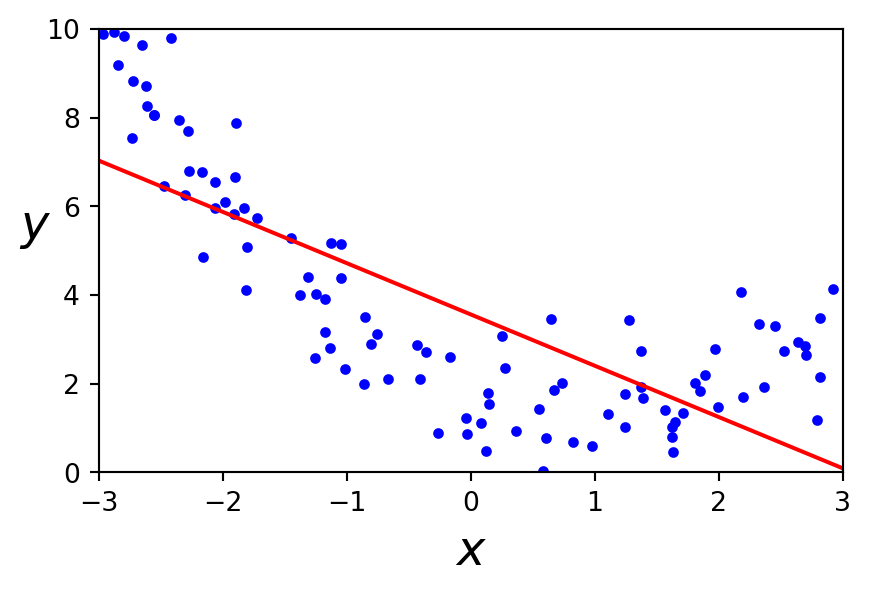
Why not MSE as a Loss Function?

What is the Difference?

Geometric Interpretation

Geometric Interpretation

• Do you recognize this equation? \[ w_1 x_1 + w_2 x_2 + \ldots + w_D x_2 \]

• This is the dot product of \(\mathbf{w}\) and \(\mathbf{x}\), \(\mathbf{w} \cdot \mathbf{x}\).

• What is the geometric interpretation of the dot product?

\[ \mathbf{w} \cdot \mathbf{x} = \|\mathbf{w}\| \|\mathbf{x}\| \cos \theta \]

In certain contexts, it is advantageous to use \(w\) in place of \(\theta\).

Geometric Interpretation

\[ \mathbf{w} \cdot \mathbf{x} = \|\mathbf{w}\| \|\mathbf{x}\| \cos \theta \]

• The dot product determines the angle \((\theta)\) between vectors.

• It quantifies how much one vector extends in the direction of another.

• Its value is zero, if the vectors are perpendicular \((\theta = 90^\circ)\).

Geometric Interpretation

• Logistic regression uses a linear combination of the input features, \(\mathbf{w} \cdot \mathbf{x} + b\), as the argument to the sigmoid (logistic) function.

• Geometrically, \(\mathbf{w}\) can be viewed as a vector normal to a hyperplane in the feature space, and any point \(\mathbf{x}\) is projected onto \(\mathbf{w}\) via the dot product \(\mathbf{w} \cdot \mathbf{x}\).

Geometric Interpretation

• The decision boundary is where this linear combination equals zero, i.e., \(\mathbf{w} \cdot \mathbf{x} + b = 0\).

• Points on one side of the boundary have a positive dot product and are more likely to be classified as the positive class (1).

• Points on the other side have a negative dot product and are more likely to be in the opposite class (0).

• The sigmoid function simply turns this signed distance into a probability between 0 and 1.

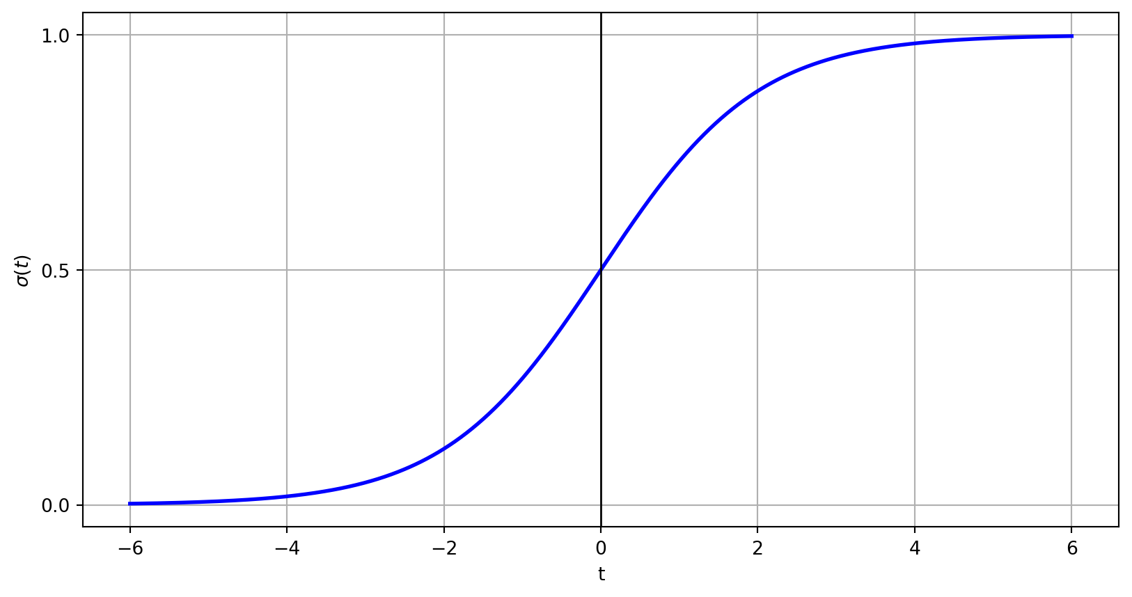
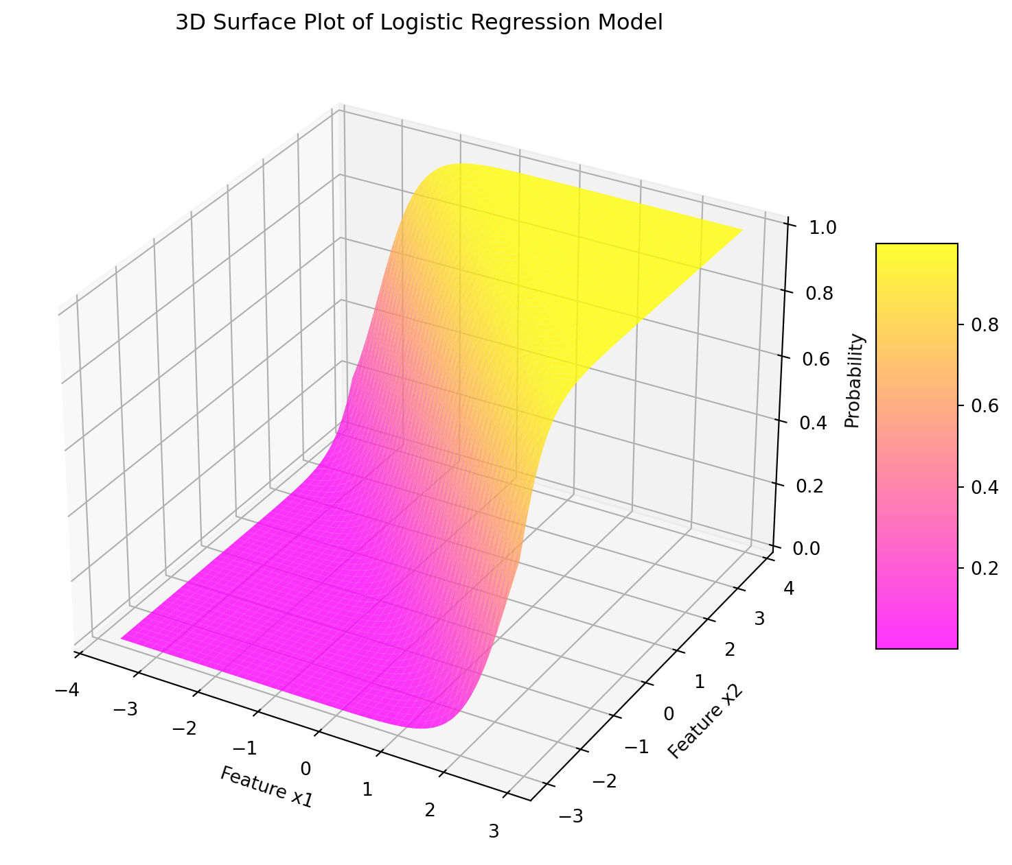
Logistic Function

\[ \sigma(t) = \frac{1}{1+e^{-t}} \]

• As \(t \to \infty\), \(e^{-t} \to 0\), so \(\sigma(t) \to 1\).
• As \(t \to -\infty\), \(e^{-t} \to \infty\), making the denominator approach infinity, so \(\sigma(t) \to 0\).
• When \(t = 0\), \(e^{-t} = 0\), resulting in a denominator of 2, so \(\sigma(t) = 0.5\).

# Sigmoid function
def sigmoid(t):
    return 1 / (1 + np.exp(-t))

# Generate t values
t = np.linspace(-6, 6, 1000)

# Compute y values for the sigmoid function
sigma = sigmoid(t)

# Create a figure
fig, ax = plt.subplots()
ax.plot(t, sigma, color='blue', linewidth=2)  # Keep the curve opaque

# Draw vertical axis at x = 0
ax.axvline(x=0, color='black', linewidth=1)

# Add labels on the vertical axis
ax.set_yticks([0, 0.5, 1.0])

# Add labels to the axes
ax.set_xlabel('t')
ax.set_ylabel(r'$\sigma(t)$')

plt.grid(True)
plt.show()

What’s special about e?

\[ \sigma(t) = \frac{1}{1+e^{-t}} \]

• Instead of \(e\), we might have used another constant, say 2.

• Derivative Simplicity: For the logistic function $(x) = $, the derivative simplifies to $’(x) = (x)(1 - (x))$. This elegant form arises because the exponential base $e$ has the unique property that $ e^x = e^x$, avoiding an extra multiplicative constant.

import math

def logistic(x, e):
    """Compute a modified logistic function using b rather than e."""
    return 1 / (1 + np.power(e, -x))

# Define a range for x values.
x = np.linspace(-6, 6, 400)

# Plot 1: Varying e.
plt.figure(figsize=(8, 6))
e_values = [2, math.e, 4, 8, 16]  # different steepness values

for e in e_values:
    plt.plot(x, logistic(x, e), label=f'e = {e}')
plt.title('Effect of Varying e')
plt.xlabel('x')
plt.ylabel(r'$\frac{1}{1+e^{-x}}$')
plt.legend()
plt.grid(True)

In the context of logistic regression, the choice of the mathematical constant \(e\) is not arbitrary but is supported by several compelling mathematical justifications. These justifications primarily relate to the harmonious integration of the logistic function with other mathematical frameworks. Although our primary focus was to visually demonstrate the potential implications of substituting a different constant, the inherent advantages of using \(e\) become evident upon closer examination of its mathematical properties and how they facilitate seamless integration with existing theories and models.

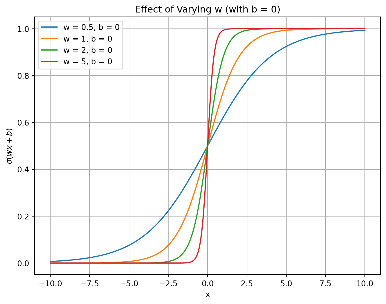
Varying w

\[ \sigma(wx + b) \]

def logistic(x, w, b):
    """Compute the logistic function with parameters w and b."""
    return 1 / (1 + np.exp(-(w * x + b)))

# Define a range for x values.
x = np.linspace(-10, 10, 400)

# Plot 1: Varying w (steepness) with b fixed at 0.
plt.figure(figsize=(8, 6))
w_values = [0.5, 1, 2, 5]  # different steepness values
b = 0  # fixed bias

for w in w_values:
    plt.plot(x, logistic(x, w, b), label=f'w = {w}, b = {b}')
plt.title('Effect of Varying w (with b = 0)')
plt.xlabel('x')
plt.ylabel(r'$\sigma(wx+b)$')
plt.legend()
plt.grid(True)
plt.show()

Varying b

\[ \sigma(wx + b) \]

# Plot 2: Varying b (horizontal shift) with w fixed at 1.
plt.figure(figsize=(8, 6))
w = 1  # fixed steepness
b_values = [-5, -2, 0, 2, 5]  # different bias values

for b in b_values:
    plt.plot(x, logistic(x, w, b), label=f'w = {w}, b = {b}')
plt.title('Effect of Varying b (with w = 1)')
plt.xlabel('x')
plt.ylabel(r'$\sigma(wx+b)$')
plt.legend()
plt.grid(True)

plt.show()

Implementation

Implementation: Generating Data

# Generate synthetic data for a binary classification problem

m = 100  # number of examples
d = 2    # number of featues

X = np.random.randn(m, d)

# Define labels using a linear decision boundary with some noise:

noise = 0.5 * np.random.randn(m)

y = (X[:, 0] + X[:, 1] + noise > 0).astype(int)

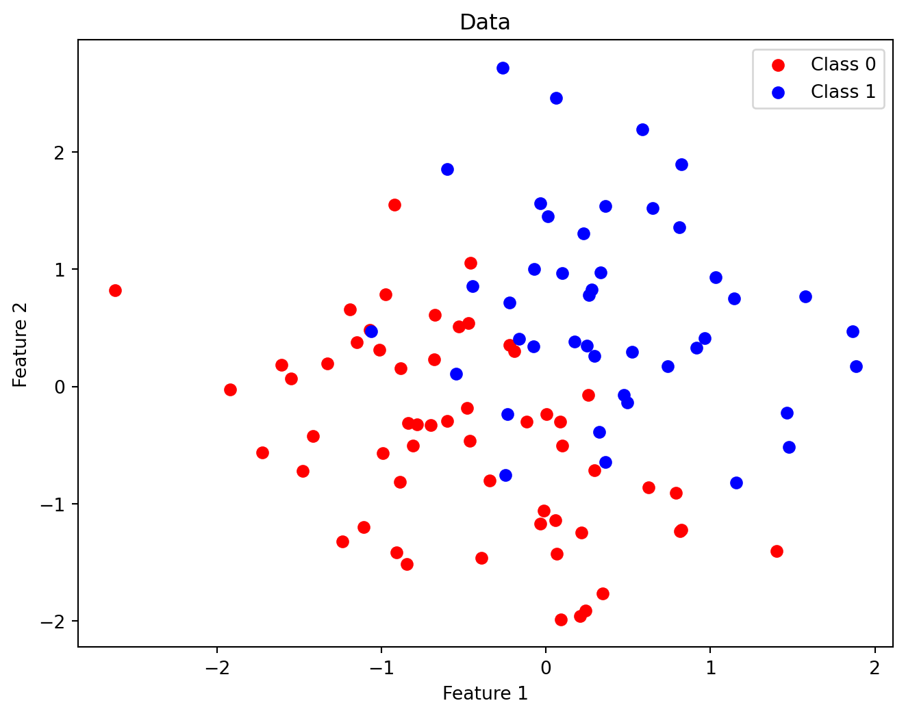
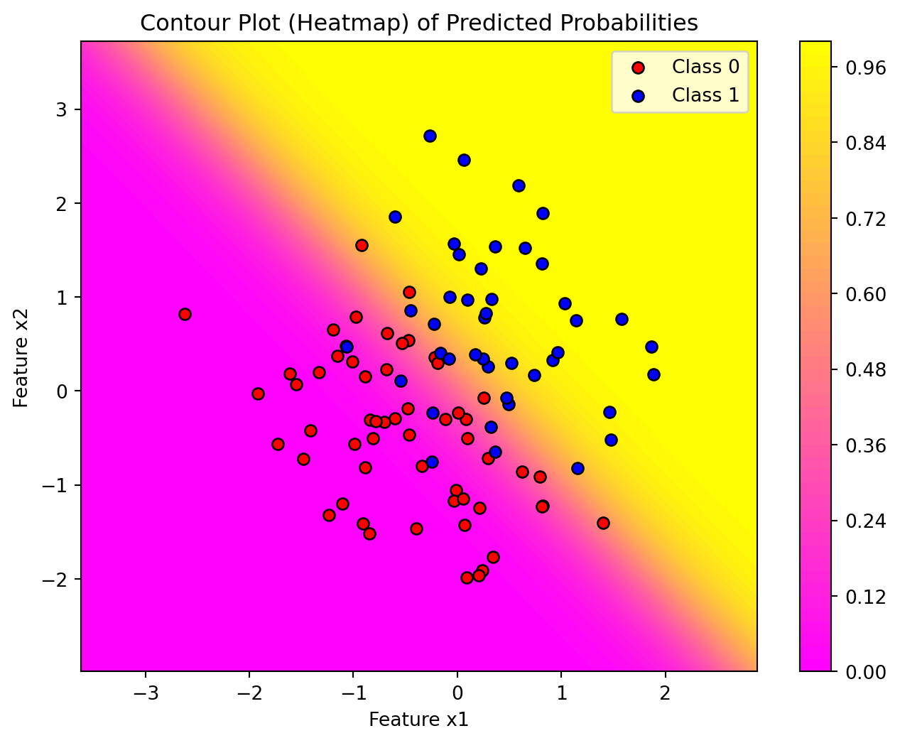
Implementation: Vizualization

# Visualize the decision boundary along with the data points
plt.figure(figsize=(8, 6))
plt.scatter(X[y == 0][:, 0], X[y == 0][:, 1], color='red', label='Class 0')
plt.scatter(X[y == 1][:, 0], X[y == 1][:, 1], color='blue', label='Class 1')

plt.xlabel("Feature 1")
plt.ylabel("Feature 2")
plt.title("Data")
plt.legend()
plt.show()

Implementation: Cost Function

# Sigmoid function
def sigmoid(z):
    return 1 / (1 + np.exp(-z))

# Cost function: binary cross-entropy
def cost_function(theta, X, y):
    m = len(y)
    h = sigmoid(X.dot(theta))
    epsilon = 1e-5  # avoid log(0)
    cost = -(1/m) * np.sum(y * np.log(h + epsilon) + (1 - y) * np.log(1 - h + epsilon))
    return cost

# Gradient of the cost function
def gradient(theta, X, y):
    m = len(y)
    h = sigmoid(X.dot(theta))
    grad = (1/m) * X.T.dot(h - y)
    return grad

Implementation: Logistic Regression

# Logistic regression training using gradient descent
def logistic_regression(X, y, learning_rate=0.1, iterations=1000):
    m, n = X.shape
    theta = np.zeros(n)
    cost_history = []
    
    for i in range(iterations):
        theta -= learning_rate * gradient(theta, X, y)
        cost_history.append(cost_function(theta, X, y))
        
    return theta, cost_history

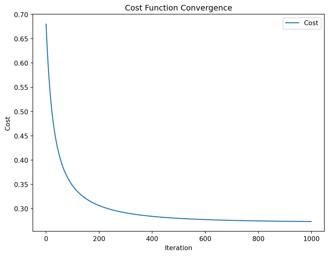
Training

# Add intercept term (bias)
X_with_intercept = np.hstack([np.ones((m, 1)), X])

# Train the logistic regression model
theta, cost_history = logistic_regression(X_with_intercept, y, learning_rate=0.1, iterations=1000)

print("Optimized theta:", theta)

Optimized theta: [-0.28840995  2.80390104  2.45238752]

Cost Function Convergence

plt.figure(figsize=(8, 6))
plt.plot(cost_history, label="Cost")
plt.xlabel("Iteration")
plt.ylabel("Cost")
plt.title("Cost Function Convergence")
plt.legend()
plt.show()

Decision Boundary and Data Points

plt.figure(figsize=(8, 6))
plt.scatter(X[y == 0][:, 0], X[y == 0][:, 1], color='red', label='Class 0')
plt.scatter(X[y == 1][:, 0], X[y == 1][:, 1], color='blue', label='Class 1')

# Decision boundary: theta0 + theta1*x1 + theta2*x2 = 0
x_vals = np.array([min(X[:, 0]) - 1, max(X[:, 0]) + 1])
y_vals = -(theta[0] + theta[1] * x_vals) / theta[2]
plt.plot(x_vals, y_vals, label='Decision Boundary', color='green')
plt.xlabel("Feature 1")
plt.ylabel("Feature 2")
plt.title("Logistic Regression Decision Boundary")
plt.legend()
plt.show()

Implementation (continued)

# Predict function: returns class labels and probabilities for new data
def predict(theta, X, threshold=0.5):
    probs = sigmoid(X.dot(theta))
    return (probs >= threshold).astype(int), probs

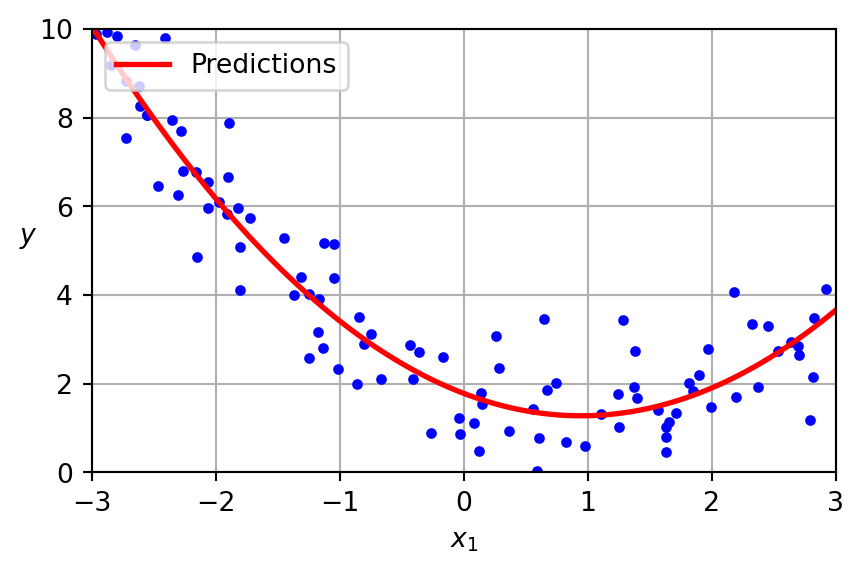
Predictions

# New examples must include the intercept term.

# Negative example (likely class 0): Choose a point far in the negative quadrant.
example_neg = np.array([1, -3, -3])

# Positive example (likely class 1): Choose a point far in the positive quadrant.
example_pos = np.array([1, 3, 3])

# Near decision boundary: Choose x1 = 0 and compute x2 from the decision boundary equation.
x1_near = 0
x2_near = -(theta[0] + theta[1] * x1_near) / theta[2]
example_near = np.array([1, x1_near, x2_near])

In the given example, each data point is characterized by two primary features. However, the representation includes three components. Why?

This discrepancy arises from an earlier discussed mathematical technique, where each instance is augmented with an additional term, \(x_i^{(0)} = 1\). This augmentation facilitates the expression of the model in a vectorized format, enhancing computational efficiency and simplicity.

Predictions (continued)

# Combine the examples into one array for prediction.
new_examples = np.vstack([example_neg, example_pos, example_near])

labels, probabilities = predict(theta, new_examples)

print("\nPredictions on new examples:")

print("Negative example {} -> Prediction: {} (Probability: {:.4f})".format(example_neg[1:], labels[0], probabilities[0]))

print("Positive example {} -> Prediction: {} (Probability: {:.4f})".format(example_pos[1:], labels[1], probabilities[1]))

print("Near-boundary example {} -> Prediction: {} (Probability: {:.4f})".format(example_near[1:], labels[2], probabilities[2]))

Predictions on new examples:
Negative example [-3 -3] -> Prediction: 0 (Probability: 0.0000)
Positive example [3 3] -> Prediction: 1 (Probability: 1.0000)
Near-boundary example [0.         0.11760374] -> Prediction: 1 (Probability: 0.5000)

Visualizing the Weight Vector

In the previous lecture, we established that logistic regression determines a weight vector that is orthogonal to the decision boundary.

Conversely, the decision boundary itself is orthogonal to the weight vector, which is derived through gradient descent optimization.

Visualizing the Weight Vector

# Plot decision boundary and data points
plt.figure(figsize=(8, 6))
plt.scatter(X[y == 0][:, 0], X[y == 0][:, 1], color='red', label='Class 0')
plt.scatter(X[y == 1][:, 0], X[y == 1][:, 1], color='blue', label='Class 1')

# Decision boundary: theta0 + theta1*x1 + theta2*x2 = 0
x_vals = np.array([min(X[:, 0]) - 1, max(X[:, 0]) + 1])
y_vals = -(theta[0] + theta[1] * x_vals) / theta[2]
plt.plot(x_vals, y_vals, label='Decision Boundary', color='green')

# --- Draw the normal vector ---
# The normal vector is (theta[1], theta[2]).
# Choose a reference point on the decision boundary. Here, we use x1 = 0:
x_ref = 0
y_ref = -theta[0] / theta[2]  # when x1=0, theta0 + theta2*x2=0  =>  x2=-theta0/theta2

# Create the normal vector from (theta[1], theta[2]).
normal = np.array([theta[1], theta[2]])

# Normalize and scale for display
normal_norm = np.linalg.norm(normal)
if normal_norm != 0:
    normal_unit = normal / normal_norm
else:
    normal_unit = normal
scale = 2  # adjust scale as needed
normal_display = normal_unit * scale

# Draw an arrow starting at the reference point
plt.arrow(x_ref, y_ref, normal_display[0], normal_display[1],
          head_width=0.1, head_length=0.2, fc='black', ec='black')
plt.text(x_ref + normal_display[0]*1.1, y_ref + normal_display[1]*1.1, 
         r'$(\theta_1, \theta_2)$', color='black', fontsize=12)

plt.xlabel("Feature 1")
plt.ylabel("Feature 2")
plt.title("Logistic Regression Decision Boundary and Normal Vector")
plt.legend()
plt.gca().set_aspect('equal', adjustable='box')
plt.ylim(-3, 3)
plt.show()

Near the Decision Boundary

# --- Visualization Setup ---
# Create a grid over the feature space
x1_range = np.linspace(X[:, 0].min()-1, X[:, 0].max()+1, 100)
x2_range = np.linspace(X[:, 1].min()-1, X[:, 1].max()+1, 100)
xx1, xx2 = np.meshgrid(x1_range, x2_range)

# Construct the grid input (with intercept) for predictions
grid = np.c_[np.ones(xx1.ravel().shape), xx1.ravel(), xx2.ravel()]
# Compute predicted probabilities over the grid
probs = sigmoid(grid.dot(theta)).reshape(xx1.shape)
# --- Approach 2: 2D Contour (Heatmap) Plot ---
plt.figure(figsize=(8, 6))
contour = plt.contourf(xx1, xx2, probs, cmap='spring', levels=50)
plt.colorbar(contour)
plt.xlabel('Feature x1')
plt.ylabel('Feature x2')
plt.title('Contour Plot (Heatmap) of Predicted Probabilities')
# Overlay training data
plt.scatter(X[y == 0][:, 0], X[y == 0][:, 1], color='red', edgecolor='k', label='Class 0')
plt.scatter(X[y == 1][:, 0], X[y == 1][:, 1], color='blue', edgecolor='k', label='Class 1')
plt.legend()
plt.show()

Near the Decision Boundary

# --- Approach 1: 3D Surface Plot ---
fig = plt.figure(figsize=(10, 8))
ax = fig.add_subplot(111, projection='3d')
surface = ax.plot_surface(xx1, xx2, probs, cmap='spring', alpha=0.8)
ax.set_xlabel('Feature x1')
ax.set_ylabel('Feature x2')
ax.set_zlabel('Probability')
ax.set_title('3D Surface Plot of Logistic Regression Model')
fig.colorbar(surface, shrink=0.5, aspect=5)
plt.show()

Prologue

Summary

In this presentation, we:

• Derived the likelihood and negative log-likelihood formulations.
• Illustrated the geometric interpretation of decision boundaries and weight vectors.
• Implemented logistic regression with gradient descent and visualized results.

Next lecture

• Performance measures and cross-evaluation

References

Russell, Stuart, and Peter Norvig. 2020. Artificial Intelligence: A Modern Approach. 4th ed. Pearson. http://aima.cs.berkeley.edu/.

Marcel Turcotte

Marcel.Turcotte@uOttawa.ca

School of Electrical Engineering and Computer Science (EECS)

University of Ottawa