Performance Evaluation

CSI 4106 - Fall 2026

Marcel Turcotte

Version: Sep 29, 2026 17:04

Preamble

Message of the Day

Lecture overview

This lecture develops classification evaluation from the confusion matrix. It introduces accuracy, precision, recall, and the F_1 score, then examines class imbalance and micro versus macro averaging. The final sections connect decision thresholds to precision-recall and ROC curves and interpret AUROC as a measure of score ranking.

Learning Objectives

  • Derive binary and one-vs-rest counts from a confusion matrix.
  • Compute and interpret accuracy, precision, recall, and the F_1 score.
  • Explain why class imbalance can make accuracy misleading.
  • Compare micro and macro averaging for multiclass metrics.
  • Relate a decision threshold to precision, recall, and an ROC operating point.
  • Construct an ROC curve from classifier scores and interpret AUROC as a ranking measure.

Performance Metrics

Confusion Matrix

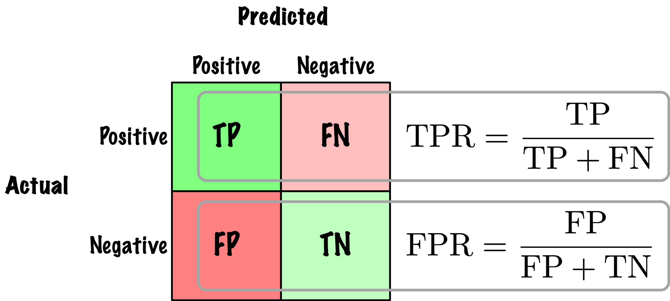
Positive (Predicted) Negative (Predicted)
Positive (Actual) True positive (TP) False negative (FN)
Negative (Actual) False positive (FP) True negative (TN)


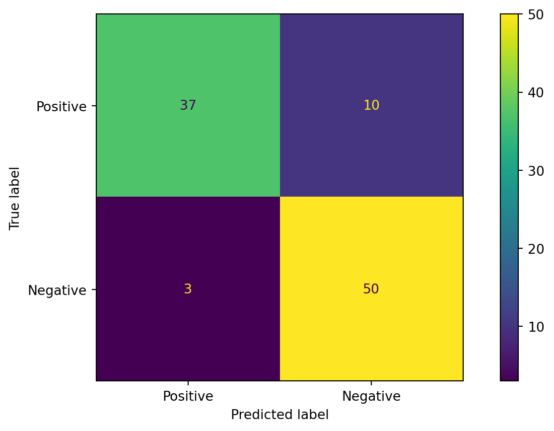
A confusion matrix is a table summarizing the performance of a classification algorithm (here for a binary classification task).

ConfusionMatrixDisplay

Code
import matplotlib.pyplot as plt
from sklearn.datasets import make_classification
from sklearn.metrics import confusion_matrix, ConfusionMatrixDisplay
from sklearn.model_selection import train_test_split
from sklearn.linear_model import LogisticRegression

seed = 42

X, y = make_classification(n_samples=500, random_state=seed)

X_train, X_test, y_train, y_test = train_test_split(
    X,
    y,
    test_size=0.2,
    random_state=seed,
    stratify=y,
)

clf = LogisticRegression(random_state=seed)

clf.fit(X_train, y_train)

predictions = clf.predict(X_test)

cm = confusion_matrix(y_test, predictions, labels=[1, 0])

disp = ConfusionMatrixDisplay(
    confusion_matrix=cm,
    display_labels=["Positive", "Negative"],
)

disp.plot()
plt.show()

Binary confusion matrix for a synthetic classification task.

Confusion Matrix

Given a test set with N examples and a classifier h(x):

C_{i,j} = \sum_{k = 1}^N [y_k = i \wedge h(x_k) = j]

Here, C is an l \times l matrix for a dataset with l classes.

Confusion Matrix

  • The total number of examples of the (actual) class i is C_{i \cdot} = \sum_{j=1}^l C_{i,j}

  • The total number of examples assigned to the (predicted) class j by classifier h is C_{\cdot j} = \sum_{i=1}^l C_{i,j}

Confusion Matrix

  • Terms on the diagonal denote the total number of examples classified correctly by classifier h. Hence, the number of correctly classified examples is \sum_{i=1}^l C_{i,i}

  • Non-diagonal terms represent misclassifications.

Confusion Matrix: Multiclass

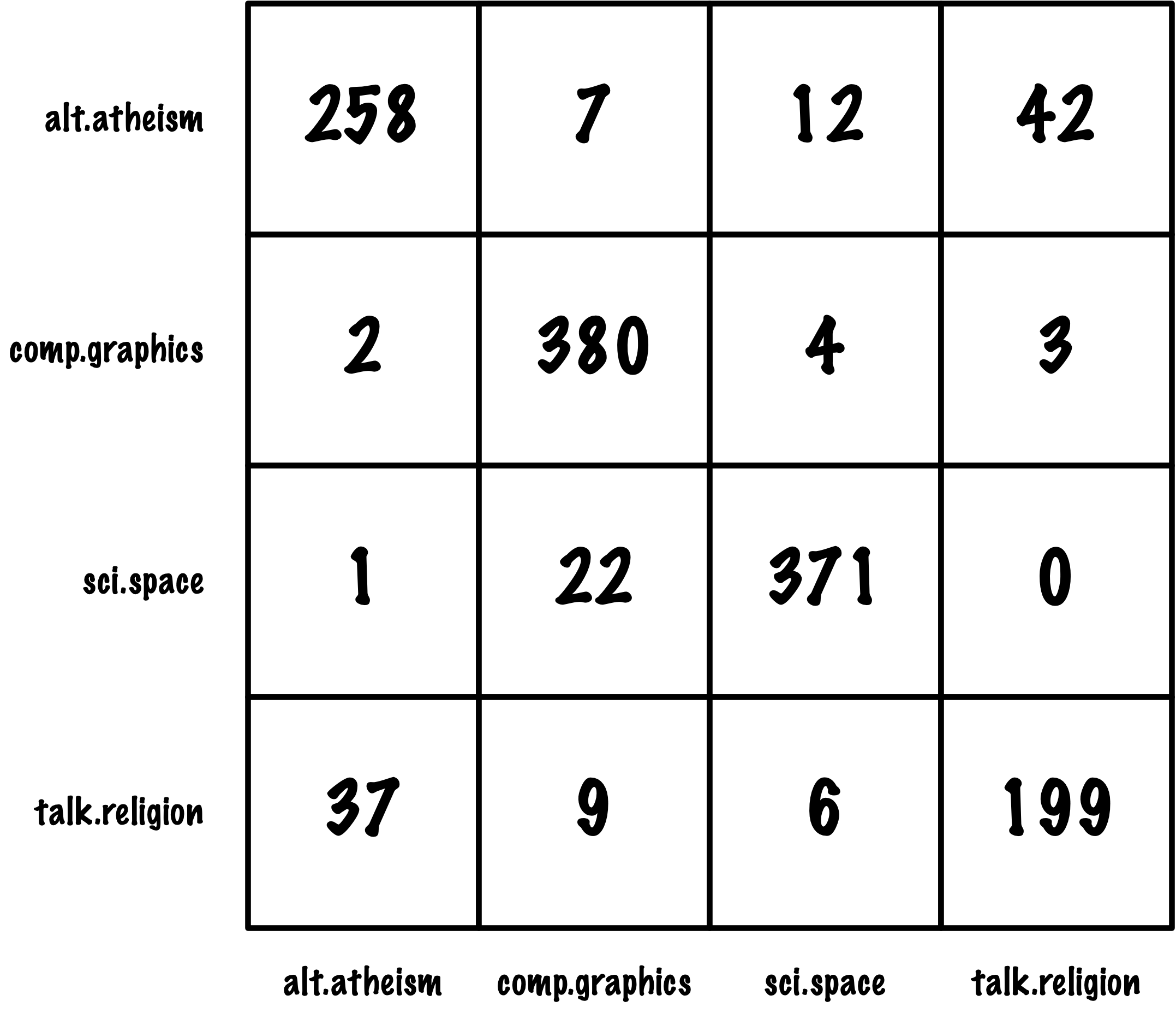
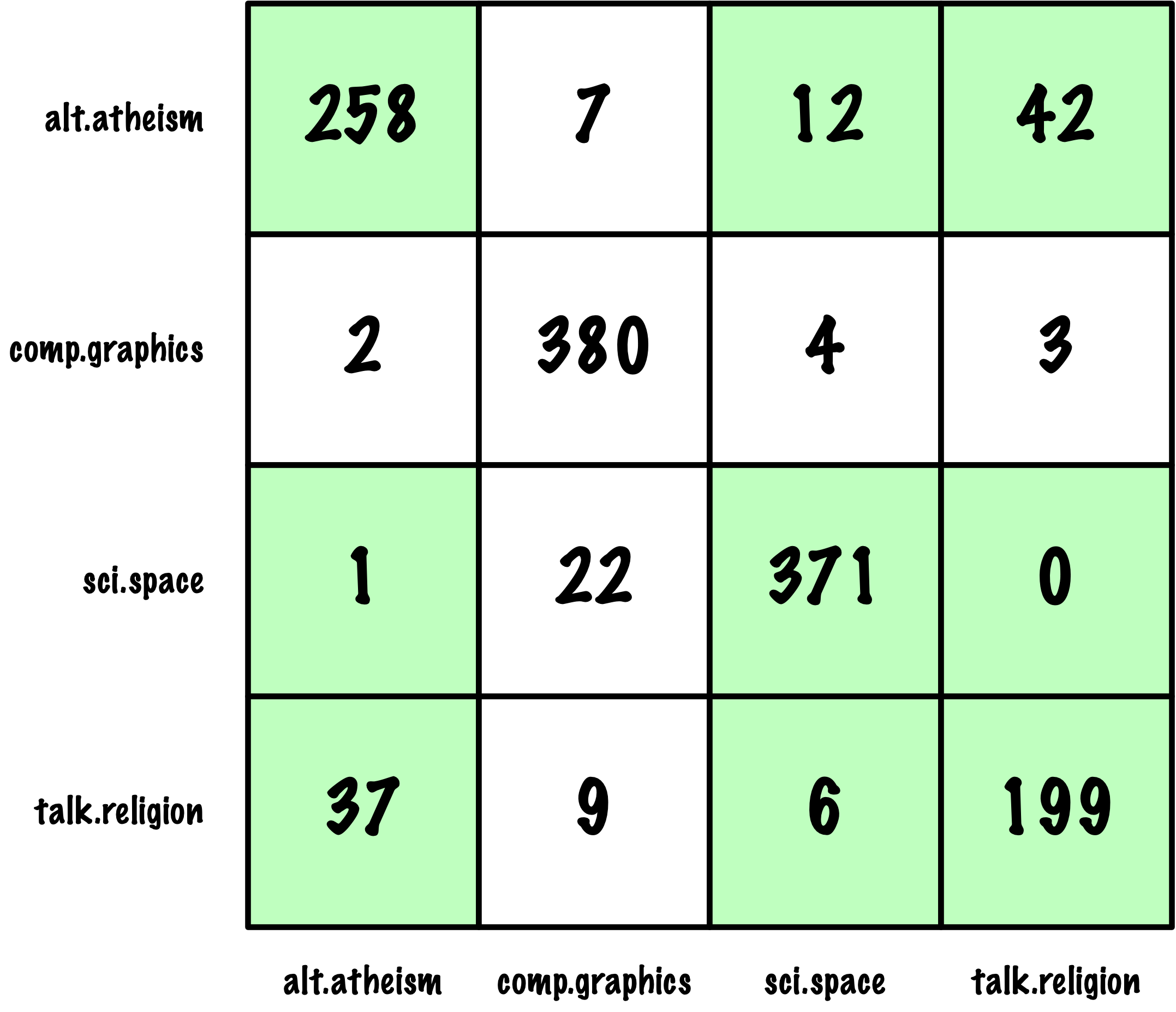
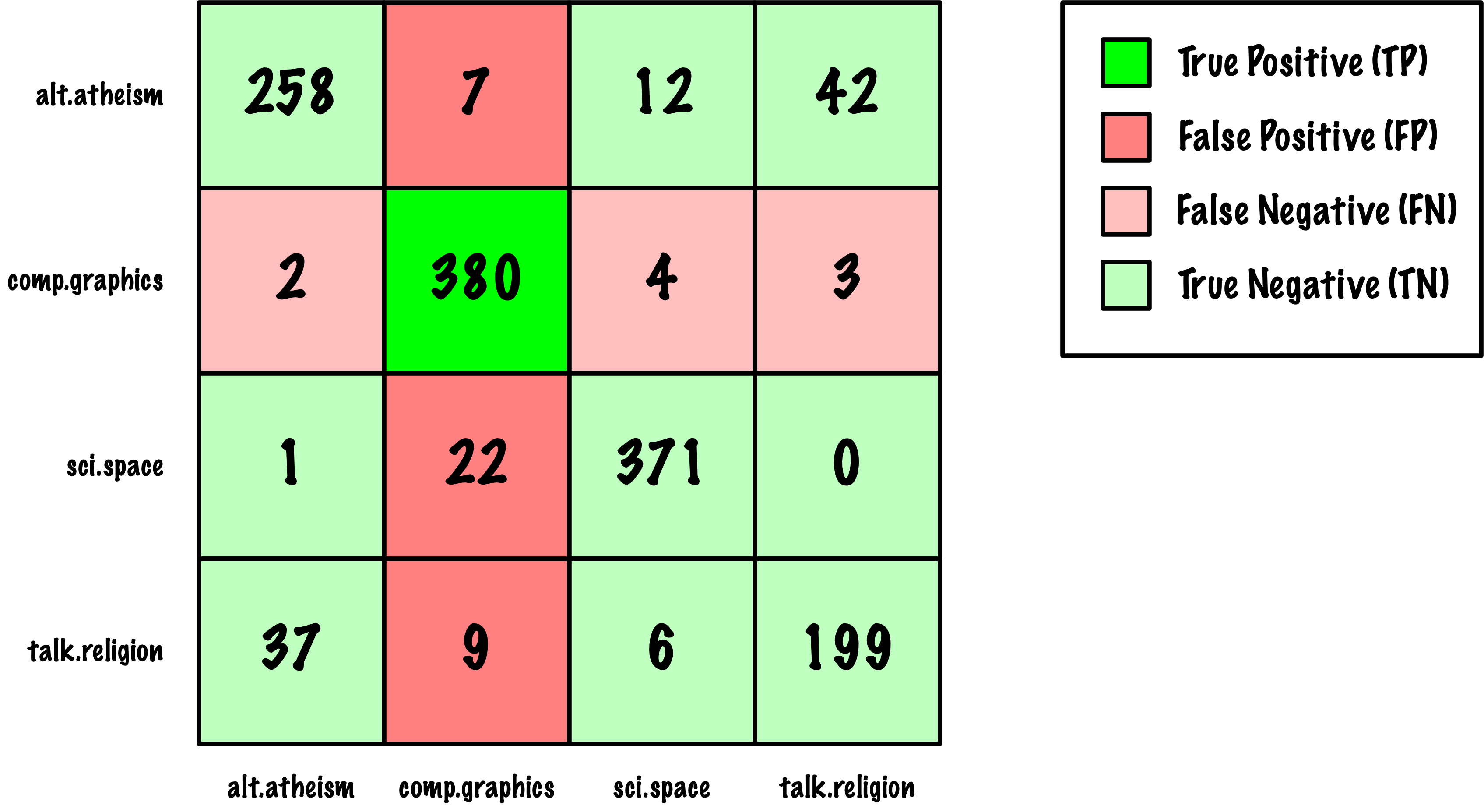
For a multiclass problem, derive one-vs-rest counts for each class and then combine the resulting class-specific metrics.

Confusion Matrix: Multiclass

Confusion Matrix: True Positive

Confusion Matrix: False Positive

Confusion Matrix: False Negative

Confusion Matrix: True Negative

Confusion Matrix: Multiclass

Multiclass counts

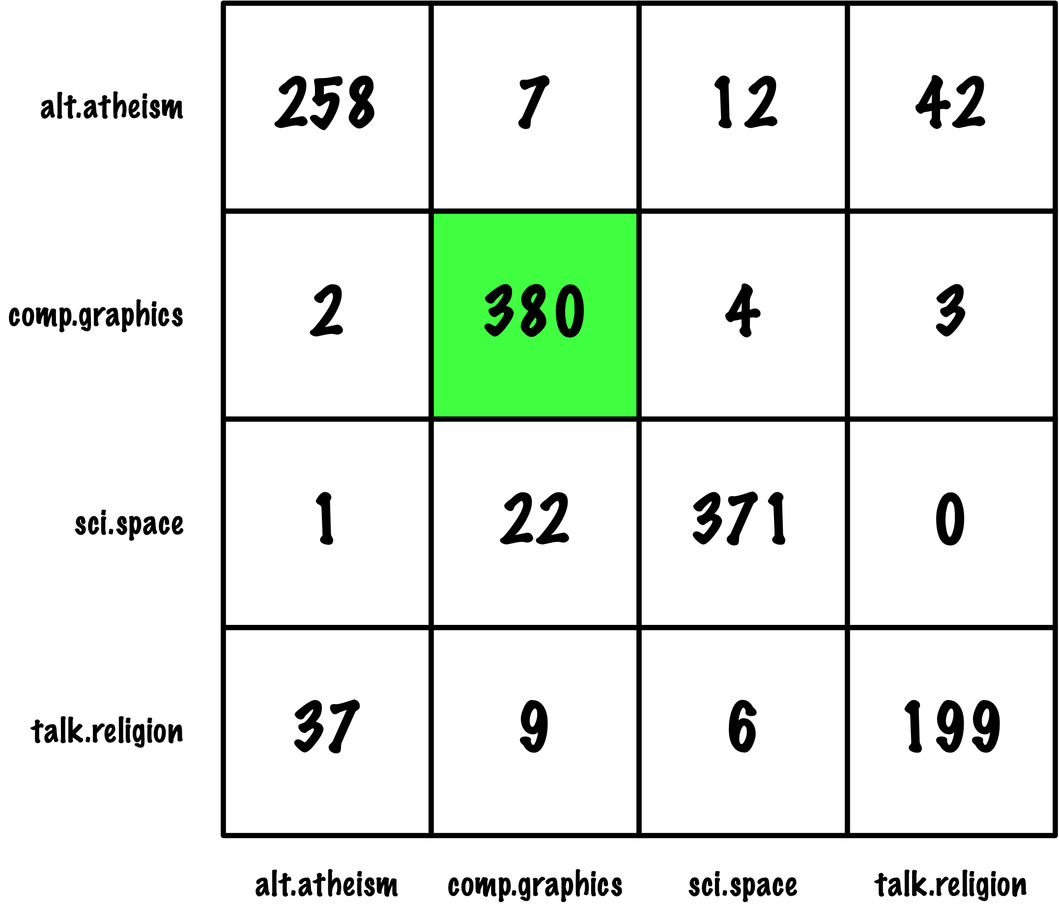
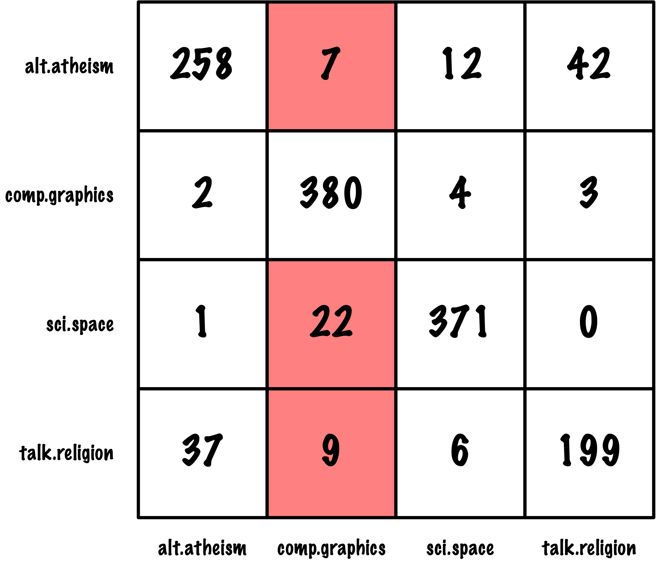
For class i, treat that class as positive and all other classes as negative:

  • True Positives (\mathrm{TP}_i): Diagonal entry C_{i,i}
  • False Positives (\mathrm{FP}_i): Sum of column i excluding C_{i,i}
  • False Negatives (\mathrm{FN}_i): Sum of row i excluding C_{i,i}
  • True Negatives (\mathrm{TN}_i): N - (\mathrm{TP}_i + \mathrm{FP}_i + \mathrm{FN}_i), equivalently \sum_{j \ne i}\sum_{k \ne i}C_{j,k}

sklearn.metrics.confusion_matrix

from sklearn.metrics import confusion_matrix

y_actual = [0, 0, 0, 1, 1, 1, 1, 1, 1, 1]
y_pred   = [0, 1, 1, 0, 0, 0, 1, 1, 1, 1]

confusion_matrix(y_actual,y_pred)
array([[1, 2],
       [3, 4]])
tn, fp, fn, tp = confusion_matrix(y_actual, y_pred).ravel().tolist()
(tn, fp, fn, tp)
(1, 2, 3, 4)

Perfect Prediction

y_actual = [0, 1, 0, 0, 1, 1, 1, 0, 1, 1]
y_pred   = [0, 1, 0, 0, 1, 1, 1, 0, 1, 1]

confusion_matrix(y_actual,y_pred)
array([[4, 0],
       [0, 6]])
tn, fp, fn, tp = confusion_matrix(y_actual, y_pred).ravel().tolist()  
(tn, fp, fn, tp)
(4, 0, 0, 6)

Confusion Matrix: Multiple Classes

Code
from sklearn.datasets import load_digits
import numpy as np

digits = load_digits()

X = digits.data
y = digits.target

X_train, X_test, y_train, y_test = train_test_split(
    X,
    y,
    test_size=0.1,
    random_state=seed,
    stratify=y,
)

from sklearn.preprocessing import StandardScaler

scaler = StandardScaler()
X_train_scaled = scaler.fit_transform(X_train)
X_test_scaled = scaler.transform(X_test)

from sklearn.multiclass import OneVsRestClassifier

clf = OneVsRestClassifier(LogisticRegression(max_iter=1000))
clf.fit(X_train_scaled, y_train)

y_pred = clf.predict(X_test_scaled)

ConfusionMatrixDisplay.from_predictions(y_test, y_pred)
plt.show()

Ten-class confusion matrix for handwritten digit predictions.

Visualizing errors

Code
mask = (y_test == 8) & (y_pred == 1)
misclassified_images = X_test[mask][:5]

plt.figure(figsize=(8, 2))
for index, image in enumerate(misclassified_images):
    plt.subplot(1, len(misclassified_images), index + 1)
    plt.imshow(np.reshape(image, (8,8)), cmap=plt.cm.gray)
    plt.title("Predicted 1")
    plt.axis("off")

plt.tight_layout()
plt.show()

Two handwritten eight that the model predicted as ones.

Accuracy

How accurate is this result?

\mathrm{accuracy} = \frac{\mathrm{TP}+\mathrm{TN}}{\mathrm{TP}+\mathrm{TN}+\mathrm{FP}+\mathrm{FN}} = \frac{\mathrm{TP}+\mathrm{TN}}{\mathrm{N}}

from sklearn.metrics import accuracy_score

y_actual = [0, 0, 0, 1, 1, 1, 1, 1, 1, 1]
y_pred   = [0, 1, 1, 0, 0, 0, 1, 1, 1, 1]

accuracy_score(y_actual,y_pred)
0.5

Accuracy

y_actual = [0, 1, 0, 0, 1, 1, 1, 0, 1, 1]
y_pred   = [1, 0, 1, 1, 0, 0, 0, 1, 0, 0]

accuracy_score(y_actual,y_pred)
0.0
y_actual = [0, 1, 0, 0, 1, 1, 1, 0, 1, 1]
y_pred   = [0, 1, 0, 0, 1, 1, 1, 0, 1, 1]

accuracy_score(y_actual,y_pred)
1.0

Accuracy can be misleading

y_actual = [0, 0, 0, 0, 1, 1, 0, 0, 0, 0]
y_pred   = [0, 0, 0, 0, 0, 0, 0, 0, 0, 0]

accuracy_score(y_actual,y_pred)
0.8

Precision

Also known as positive predictive value (PPV).

\mathrm{precision} = \frac{\mathrm{TP}}{\mathrm{TP}+\mathrm{FP}}

from sklearn.metrics import precision_score

y_actual = [0, 0, 0, 1, 1, 1, 1, 1, 1, 1]
y_pred   = [0, 1, 1, 0, 0, 0, 1, 1, 1, 1]

precision_score(y_actual, y_pred)
0.6666666666666666

Precision alone is not enough

y_actual = [0, 0, 0, 1, 1, 1, 1, 1, 1, 1]
y_pred   = [0, 0, 0, 0, 0, 0, 1, 0, 0, 0]

precision_score(y_actual,y_pred)
1.0

Recall

Also known as sensitivity or true positive rate (TPR). \mathrm{recall} = \frac{\mathrm{TP}}{\mathrm{TP}+\mathrm{FN}}

from sklearn.metrics import recall_score

y_actual = [0, 0, 0, 1, 1, 1, 1, 1, 1, 1]
y_pred   = [0, 1, 1, 0, 0, 0, 1, 1, 1, 1]

recall_score(y_actual,y_pred)
0.5714285714285714

F_1 score

\begin{align*} F_1~\mathrm{score} &= \frac{2}{\frac{1}{\mathrm{precision}}+\frac{1}{\mathrm{recall}}} = 2 \times \frac{\mathrm{precision}\times\mathrm{recall}}{\mathrm{precision}+\mathrm{recall}} \\ &= \frac{\mathrm{TP}}{\mathrm{TP}+\frac{\mathrm{FN}+\mathrm{FP}}{2}} \end{align*}

from sklearn.metrics import f1_score

y_actual = [0, 0, 0, 1, 1, 1, 1, 1, 1, 1]
y_pred   = [0, 1, 1, 0, 0, 0, 1, 1, 1, 1]

f1_score(y_actual,y_pred)
0.6153846153846154

Micro and Macro Averaging

Definition

The class imbalance problem occurs when one class has substantially more examples than another.

Without appropriate training and evaluation choices, a model may favour the majority class and perform poorly on the minority class.

Micro Performance Metrics

  • Micro averaging pools the true positives, false positives, and false negatives across classes before computing precision, recall, or F_1.
  • It treats each prediction equally, so frequent classes contribute more to the final metric.

Macro Performance Metrics

  • Macro averaging computes the metric independently for each class and then takes the arithmetic mean.
  • It treats each class equally, regardless of its frequency, so poor performance on an infrequent class remains visible.

Multiclass metrics

When calculating precision, recall, and F_1, one usually computes one-vs-rest metrics for each class and then averages them using a micro or macro scheme.

  • True Positives (\mathrm{TP}_i): Diagonal entry C_{i,i}
  • False Positives (\mathrm{FP}_i): Sum of column i excluding C_{i,i}
  • False Negatives (\mathrm{FN}_i): Sum of row i excluding C_{i,i}
  • True Negatives (\mathrm{TN}_i): N - (\mathrm{TP}_i + \mathrm{FP}_i + \mathrm{FN}_i)

Multiclass formulas

When calculating precision, recall, and F_1, one usually computes one-vs-rest metrics for each class and then averages them using a micro or macro scheme.

  • \mathrm{TP}_i = C_{i,i}
  • \mathrm{FP}_i = \sum_{k \ne i} C_{k,i}
  • \mathrm{FN}_i = \sum_{k \ne i} C_{i,k}
  • \mathrm{TN}_i = \sum_{j \ne i} \sum_{k \ne i} C_{j,k}

Micro/Macro Metrics

# Sample data
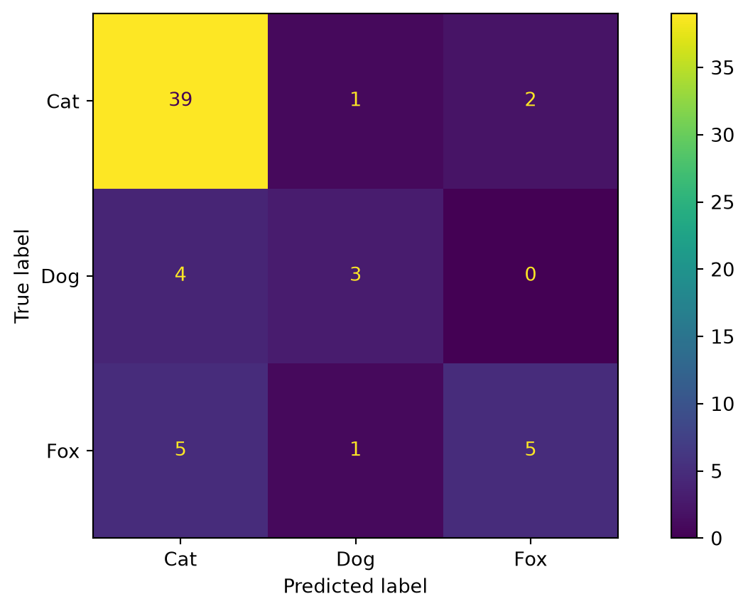
y_true = ['Cat'] * 42 + ['Dog'] *  7 + ['Fox'] * 11
y_pred = ['Cat'] * 39 + ['Dog'] *  1 + ['Fox'] *  2 + \
         ['Cat'] *  4 + ['Dog'] *  3 + ['Fox'] *  0 + \
         ['Cat'] *  5 + ['Dog'] *  1 + ['Fox'] *  5

ConfusionMatrixDisplay.from_predictions(y_true, y_pred)

Three-class confusion matrix for cats, dogs, and foxes.

Micro/Macro Precision

from sklearn.metrics import classification_report, precision_score

print(classification_report(y_true, y_pred), "\n")

micro_precision = precision_score(y_true, y_pred, average="micro")
macro_precision = precision_score(y_true, y_pred, average="macro")
print(f"Micro precision: {micro_precision:.2f}")
print(f"Macro precision: {macro_precision:.2f}")
              precision    recall  f1-score   support

         Cat       0.81      0.93      0.87        42
         Dog       0.60      0.43      0.50         7
         Fox       0.71      0.45      0.56        11

    accuracy                           0.78        60
   macro avg       0.71      0.60      0.64        60
weighted avg       0.77      0.78      0.77        60
 

Micro precision: 0.78
Macro precision: 0.71

Micro/Macro Precision

  • Macro-average precision is calculated as the mean of the precision scores1 for each class: \frac{0.81 + 0.60 + 0.71}{3} = 0.71.

  • Micro-average precision pools the counts from the entire confusion matrix: \frac{TP}{TP+FP} = \frac{39+3+5}{39+3+5+9+2+2} = \frac{47}{60} = 0.78.

Micro/Macro Recall

from sklearn.metrics import classification_report, recall_score

print(classification_report(y_true, y_pred), "\n")

micro_recall = recall_score(y_true, y_pred, average="micro")
macro_recall = recall_score(y_true, y_pred, average="macro")
print(f"Micro recall: {micro_recall:.2f}")
print(f"Macro recall: {macro_recall:.2f}")
              precision    recall  f1-score   support

         Cat       0.81      0.93      0.87        42
         Dog       0.60      0.43      0.50         7
         Fox       0.71      0.45      0.56        11

    accuracy                           0.78        60
   macro avg       0.71      0.60      0.64        60
weighted avg       0.77      0.78      0.77        60
 

Micro recall: 0.78
Macro recall: 0.60

Micro/Macro Recall

  • Macro-average recall is calculated as the mean of the recall scores for each class: \frac{0.93 + 0.43 + 0.45}{3} = 0.60.

  • Micro-average recall pools the counts from the entire confusion matrix: \frac{TP}{TP+FN} = \frac{39+3+5}{39+3+5+3+4+6} = \frac{47}{60} = 0.78.

Class Imbalance in Medical Data

Micro/Macro Metrics (Medical Data)

Code
# Sample data
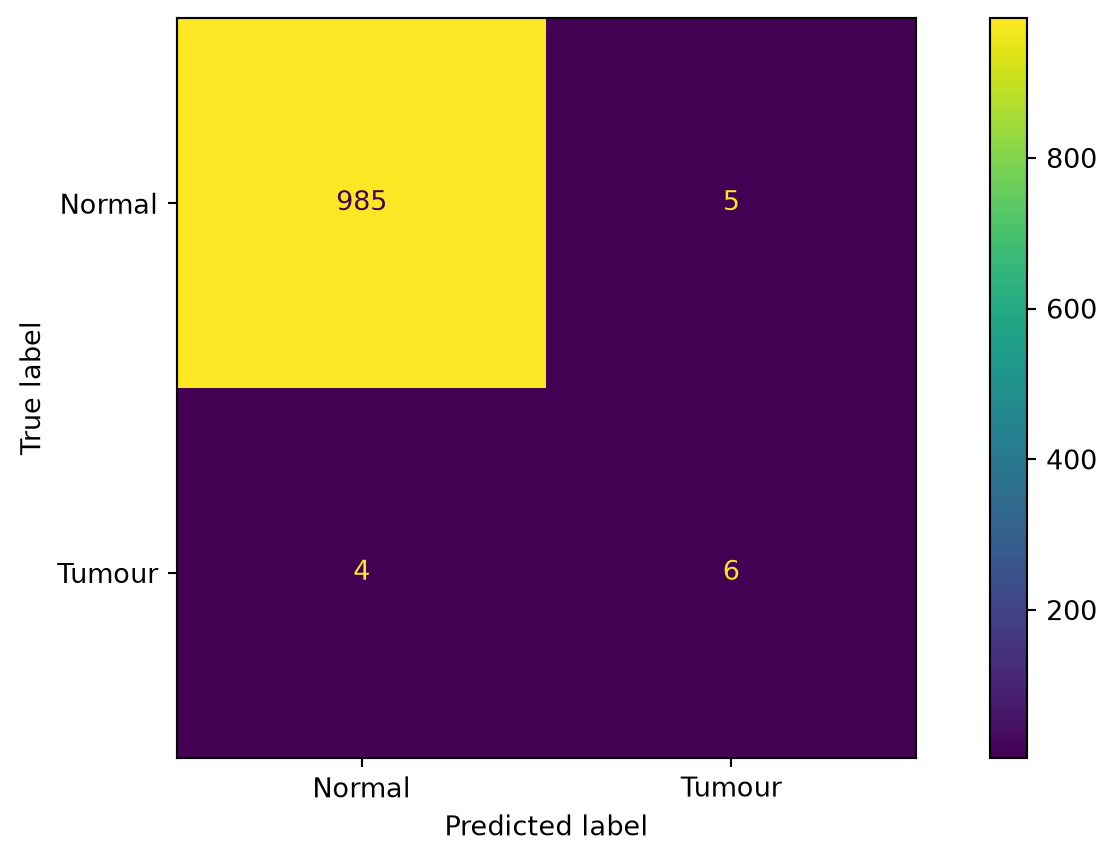
y_true = ['Normal'] *  990 + ['Tumour'] *  10
y_pred = ['Normal'] *  985 + ['Tumour'] *   5 + \
         ['Normal'] *    4 + ['Tumour'] *   6

ConfusionMatrixDisplay.from_predictions(y_true, y_pred)

Confusion matrix for an imbalanced medical example.

Micro/macro metrics (medical data)

from sklearn.metrics import classification_report, recall_score

print(classification_report(y_true, y_pred), "\n")

micro_precision = precision_score(y_true, y_pred, average="micro")
macro_precision = precision_score(y_true, y_pred, average="macro")
print(f"Micro precision: {micro_precision:.2f}")
print(f"Macro precision: {macro_precision:.2f}")

print("\n")

micro_recall = recall_score(y_true, y_pred, average="micro")
macro_recall = recall_score(y_true, y_pred, average="macro")
print(f"Micro recall: {micro_recall:.2f}")
print(f"Macro recall: {macro_recall:.2f}")

Micro/macro metrics (medical data)

              precision    recall  f1-score   support

      Normal       1.00      0.99      1.00       990
      Tumour       0.55      0.60      0.57        10

    accuracy                           0.99      1000
   macro avg       0.77      0.80      0.78      1000
weighted avg       0.99      0.99      0.99      1000
 

Micro precision: 0.99
Macro precision: 0.77


Micro recall: 0.99
Macro recall: 0.80

Precision-Recall Trade-Off

Handwritten Digits (Revisited)

Loading the dataset

Code
from sklearn.datasets import fetch_openml

digits = fetch_openml('mnist_784', as_frame=False)
X, y = digits.data, digits.target

Plotting the first five examples

Code
plt.figure(figsize=(10,2))
n = 5

for index, (image, label) in enumerate(zip(X[0:n], y[0:n])):
    plt.subplot(1, n, index + 1)
    plt.imshow(np.reshape(image, (28,28)), cmap=plt.cm.gray)
    plt.title(f'y = {label}')

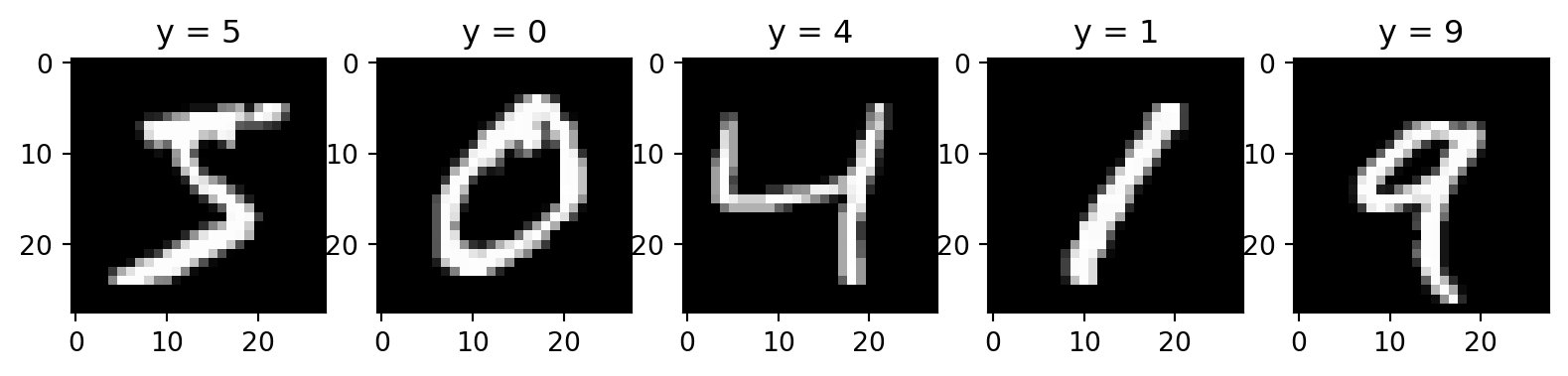
Five sample handwritten digits from the MNIST dataset.

These images have dimensions of 28 \times 28 pixels.

Creating a Binary Classification Task

# Creating a binary classification task (one vs the rest)

some_digit = X[0]
some_digit_y = y[0]

y = (y == some_digit_y)
y
array([ True, False, False, ..., False,  True, False], shape=(70000,))
# Creating the training and test sets
X_train, X_test, y_train, y_test = train_test_split(
    X,
    y,
    test_size=0.1,
    random_state=seed,
    stratify=y,
)

SGDClassifier

from sklearn.linear_model import SGDClassifier

clf = SGDClassifier(random_state=seed)

clf.fit(X_train, y_train)

Performance

y_pred = clf.predict(X_test)

accuracy_score(y_test, y_pred)
0.9657142857142857

The score appears strong,

but the class distribution provides essential context.

Not so Fast

from sklearn.dummy import DummyClassifier

dummy_clf = DummyClassifier(strategy="most_frequent")

dummy_clf.fit(X_train, y_train)
y_pred = dummy_clf.predict(X_test)

accuracy_score(y_test, y_pred)
0.9098571428571428

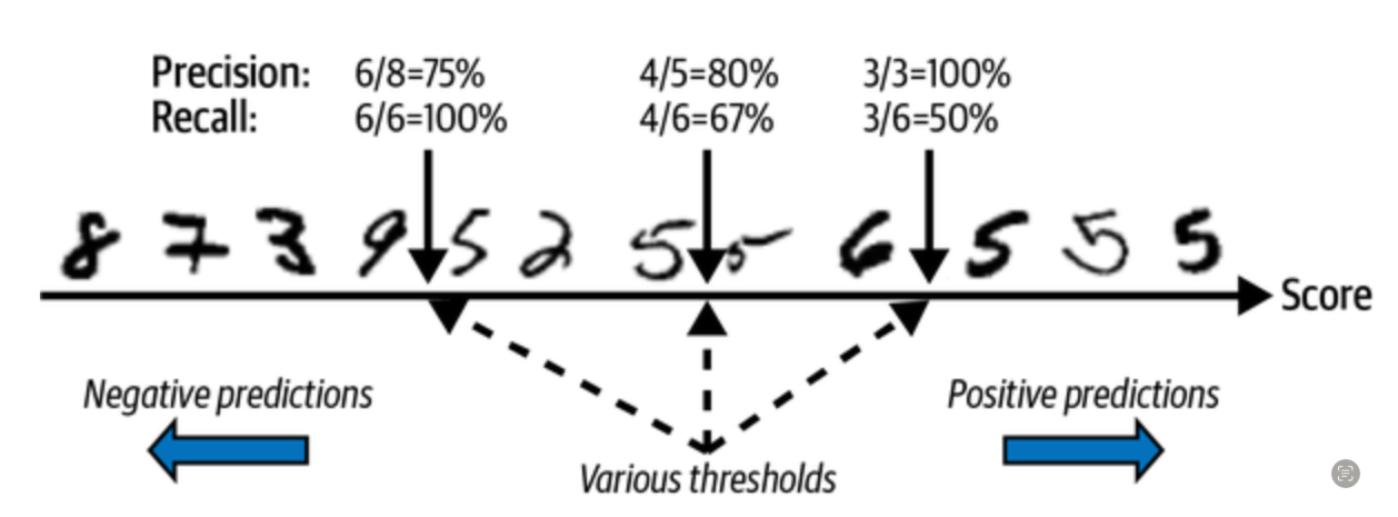
Precision-Recall Trade-Off

Precision-Recall Trade-Off

Code
from sklearn.model_selection import cross_val_predict
y_scores = cross_val_predict(
    clf,
    X_train,
    y_train,
    cv=3,
    method="decision_function",
)

from sklearn.metrics import precision_recall_curve

precisions, recalls, thresholds = precision_recall_curve(
    y_train,
    y_scores,
)

threshold = 3000

plt.figure(figsize=(8, 4))
plt.plot(
    thresholds,
    precisions[:-1],
    "b--",
    label="Precision",
    linewidth=2,
)
plt.plot(thresholds, recalls[:-1], "g-", label="Recall", linewidth=2)
plt.vlines(threshold, 0, 1.0, "k", "dotted", label="threshold")

idx = (thresholds >= threshold).argmax()  # first index ≥ threshold
plt.plot(thresholds[idx], precisions[idx], "bo")
plt.plot(thresholds[idx], recalls[idx], "go")
plt.axis([-50000, 50000, 0, 1])
plt.grid()
plt.xlabel("Threshold")
plt.legend(loc="center right")

plt.show()

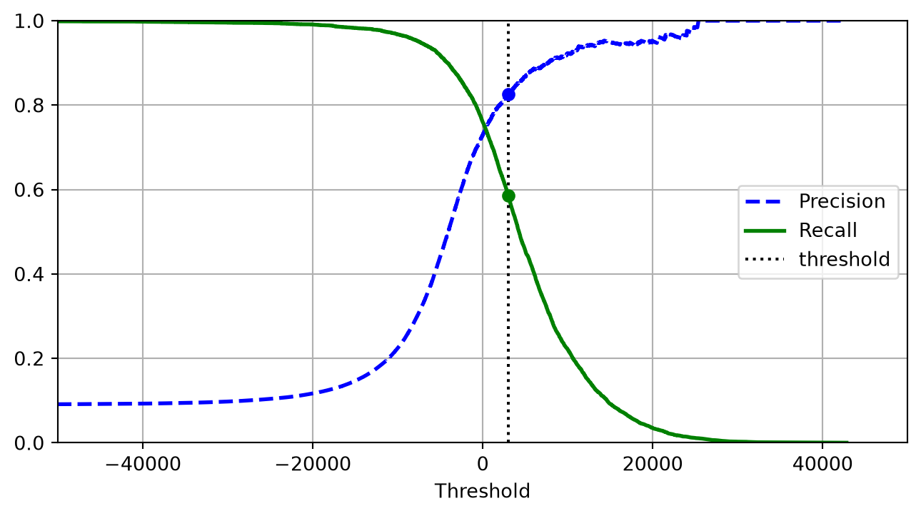
Precision and recall as functions of the decision threshold.

Precision/Recall Curve

Code
import matplotlib.patches as patches

plt.figure(figsize=(5, 5))

plt.plot(
    recalls,
    precisions,
    linewidth=2,
    label="Precision/Recall Curve",
)

plt.plot([recalls[idx], recalls[idx]], [0., precisions[idx]], "k:")
plt.plot([0.0, recalls[idx]], [precisions[idx], precisions[idx]], "k:")
plt.plot([recalls[idx]], [precisions[idx]], "ko",
         label="Point at threshold 3,000")
plt.gca().add_patch(patches.FancyArrowPatch(
    (0.79, 0.60), (0.61, 0.78),
    connectionstyle="arc3,rad=.2",
    arrowstyle="Simple, tail_width=1.5, head_width=8, head_length=10",
    color="#444444"))
plt.text(0.56, 0.62, "Higher\nthreshold", color="#333333")
plt.xlabel("Recall")
plt.ylabel("Precision")
plt.axis([0, 1, 0, 1])
plt.grid()
plt.legend(loc="lower left")

plt.show()

Precision-recall curve with one selected threshold marked.

ROC Curve

ROC Curve

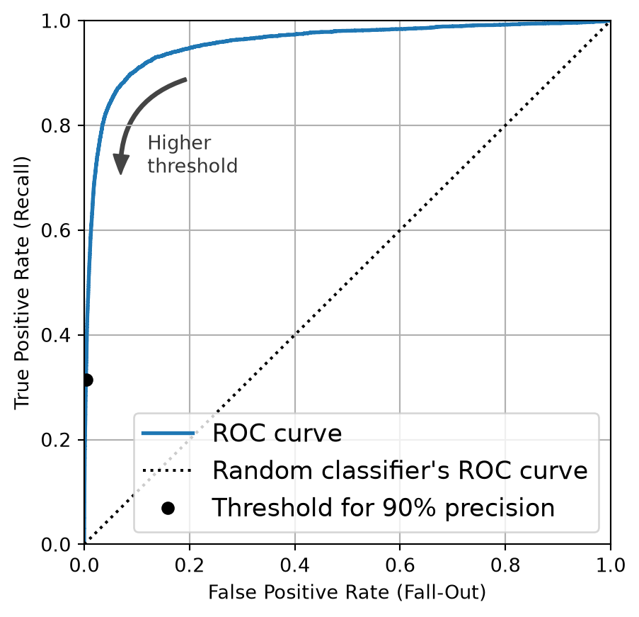
Receiver operating characteristic (ROC) curve

  • True positive rate (TPR) against false positive rate (FPR)
  • An ideal classifier has TPR close to 1.0 and FPR close to 0.0
  • \mathrm{TPR} = \frac{\mathrm{TP}}{\mathrm{TP}+\mathrm{FN}} (recall, sensitivity)
  • TPR approaches one when there are few false negatives
  • \mathrm{FPR} = \frac{\mathrm{FP}}{\mathrm{FP}+\mathrm{TN}} = 1-\mathrm{specificity}
  • FPR approaches zero when the number of false positives is low

ROC Curve

ROC Curve

Code
idx_for_90_precision = (precisions >= 0.90).argmax()
threshold_for_90_precision = thresholds[idx_for_90_precision]
y_train_pred_90 = (y_scores >= threshold_for_90_precision)

from sklearn.metrics import roc_curve

fpr, tpr, thresholds = roc_curve(y_train, y_scores)

idx_for_threshold_at_90 = (
    thresholds <= threshold_for_90_precision
).argmax()
tpr_90 = tpr[idx_for_threshold_at_90]
fpr_90 = fpr[idx_for_threshold_at_90]

plt.figure(figsize=(5, 5))
plt.plot(fpr, tpr, linewidth=2, label="ROC curve")
plt.plot([0, 1], [0, 1], 'k:', label="Random classifier's ROC curve")
plt.plot([fpr_90], [tpr_90], "ko", label="Threshold for 90% precision")

plt.gca().add_patch(patches.FancyArrowPatch(
    (0.20, 0.89), (0.07, 0.70),
    connectionstyle="arc3,rad=.4",
    arrowstyle="Simple, tail_width=1.5, head_width=8, head_length=10",
    color="#444444"))
plt.text(0.12, 0.71, "Higher\nthreshold", color="#333333")
plt.xlabel('False Positive Rate (Fall-Out)')
plt.ylabel('True Positive Rate (Recall)')
plt.grid()
plt.axis([0, 1, 0, 1])
plt.legend(loc="lower right", fontsize=13)

plt.show()

ROC curve with the operating point for 90 percent precision.

Score distributions and the ROC curve

Code
from sklearn.metrics import roc_auc_score, roc_curve

def plot_scores_and_roc(
    ax_scores,
    ax_roc,
    negative_scores,
    positive_scores,
    title,
    threshold=None,
):
    """Plot class score distributions beside their ROC curve."""
    labels = np.concatenate([
        np.zeros(len(negative_scores), dtype=int),
        np.ones(len(positive_scores), dtype=int),
    ])
    scores = np.concatenate([negative_scores, positive_scores])

    bins = np.linspace(0, 1, 21)
    ax_scores.hist(
        negative_scores,
        bins=bins,
        alpha=0.6,
        label="Negative examples",
    )
    ax_scores.hist(
        positive_scores,
        bins=bins,
        alpha=0.6,
        label="Positive examples",
    )
    ax_scores.set(
        title=title,
        xlabel="Prediction score",
        ylabel="Number of examples",
        xlim=(0, 1),
    )

    curve_fpr, curve_tpr, _ = roc_curve(labels, scores)
    area = roc_auc_score(labels, scores)
    ax_roc.plot(curve_fpr, curve_tpr, linewidth=2, label="ROC curve")
    ax_roc.plot([0, 1], [0, 1], "k--", label="Random ranking")
    ax_roc.set(
        title=f"AUROC = {area:.2f}",
        xlabel="False-positive rate",
        ylabel="True-positive rate",
        xlim=(0, 1),
        ylim=(0, 1),
    )
    ax_roc.set_aspect("equal", adjustable="box")

    if threshold is not None:
        predictions = (scores >= threshold).astype(int)
        tn, fp, fn, tp = confusion_matrix(
            labels,
            predictions,
            labels=[0, 1],
        ).ravel()
        point_fpr = fp / (fp + tn)
        point_tpr = tp / (tp + fn)
        accuracy = np.mean(predictions == labels)

        ax_scores.axvline(
            threshold,
            color="black",
            linestyle=":",
            label=f"Threshold = {threshold:.2f}",
        )
        ax_scores.text(
            0.02,
            0.95,
            f"Accuracy = {accuracy:.2f}",
            transform=ax_scores.transAxes,
            va="top",
        )
        ax_roc.scatter(
            point_fpr,
            point_tpr,
            color="black",
            zorder=3,
            label="Selected threshold",
        )

    ax_scores.legend(fontsize=8)
    ax_roc.legend(fontsize=8, loc="lower right")


roc_demo_rng = np.random.default_rng(seed)
roc_demo_size = 250
good_negative_scores = np.clip(
    roc_demo_rng.normal(0.35, 0.16, roc_demo_size),
    0,
    1,
)
good_positive_scores = np.clip(
    roc_demo_rng.normal(0.65, 0.16, roc_demo_size),
    0,
    1,
)

fig, axes = plt.subplots(1, 2, figsize=(10, 4.5), constrained_layout=True)
plot_scores_and_roc(
    axes[0],
    axes[1],
    good_negative_scores,
    good_positive_scores,
    "Overlapping score distributions",
    threshold=0.50,
)
plt.show()

Score distributions and the ROC curve

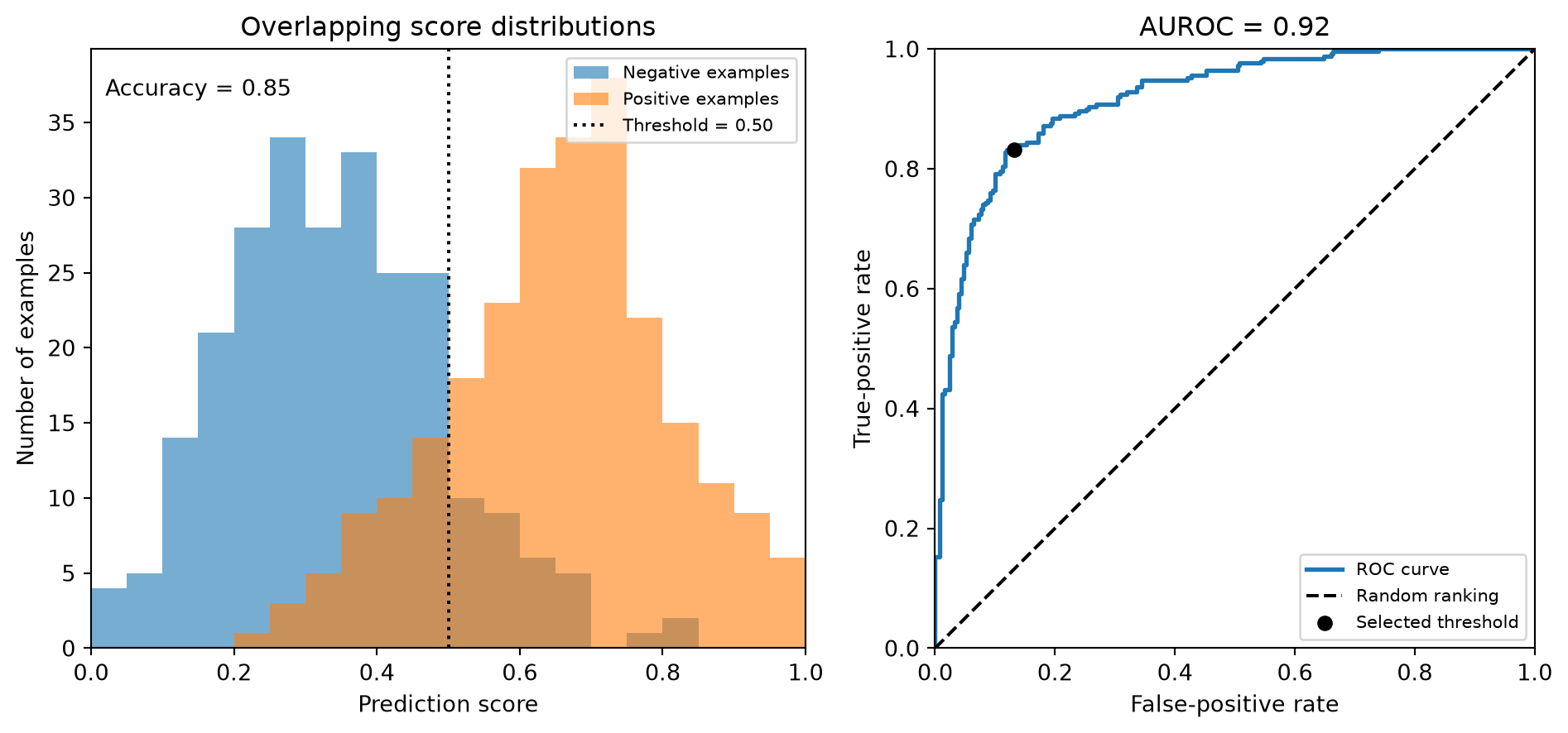
Prediction-score histograms for the negative and positive classes beside the corresponding ROC curve, with one threshold marked in both plots.

Area under the ROC curve

The area under the ROC curve (AUROC) summarizes how well a score ranks positive examples above negative examples.

  • \mathrm{AUROC}=1: every positive example receives a higher score than every negative example.
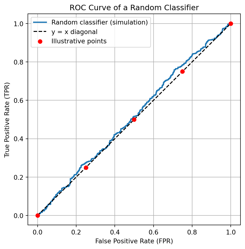
  • \mathrm{AUROC}=0.5: random ranking on average.
  • \mathrm{AUROC}<0.5: the ranking is systematically reversed.

AUROC compares rankings across thresholds. It does not measure probability calibration and does not choose an operating threshold.

Perfect classifier

Code
perfect_rng = np.random.default_rng(seed + 1)
perfect_negative_scores = np.clip(
    perfect_rng.normal(0.25, 0.07, roc_demo_size),
    0,
    1,
)
perfect_positive_scores = np.clip(
    perfect_rng.normal(0.75, 0.07, roc_demo_size),
    0,
    1,
)

fig, axes = plt.subplots(1, 2, figsize=(10, 4.5), constrained_layout=True)
plot_scores_and_roc(
    axes[0],
    axes[1],
    perfect_negative_scores,
    perfect_positive_scores,
    "Separated Gaussian score distributions",
)
plt.show()
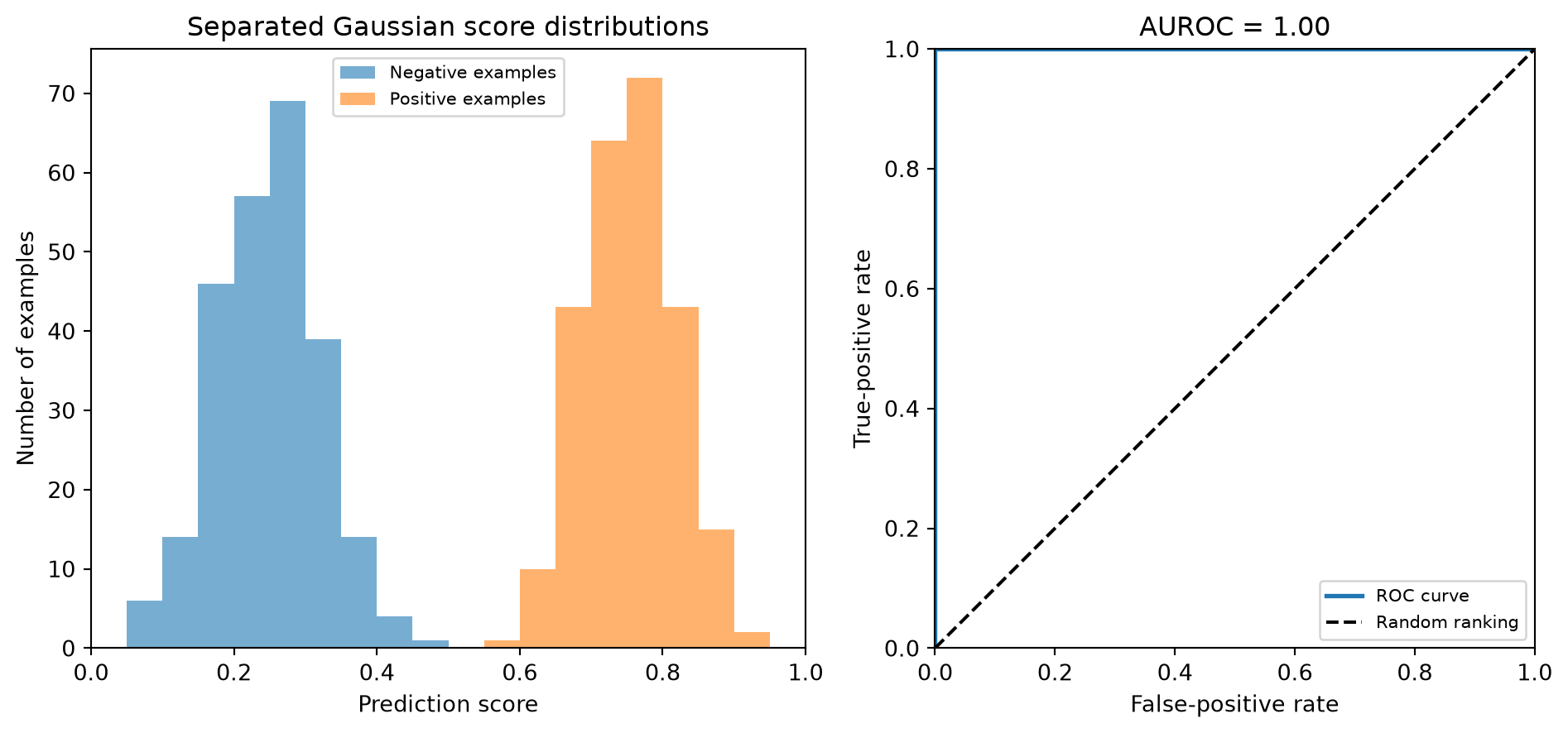
Perfect classifier

Separated Gaussian score distributions for negative and positive examples beside a perfect ROC curve.

Random classifier

Code
random_rng = np.random.default_rng(seed + 2)
random_negative_scores = random_rng.uniform(0.05, 0.95, roc_demo_size)
random_positive_scores = random_rng.uniform(0.05, 0.95, roc_demo_size)

fig, axes = plt.subplots(1, 2, figsize=(10, 4.5), constrained_layout=True)
plot_scores_and_roc(
    axes[0],
    axes[1],
    random_negative_scores,
    random_positive_scores,
    "Independent uniform score samples",
)
plt.show()
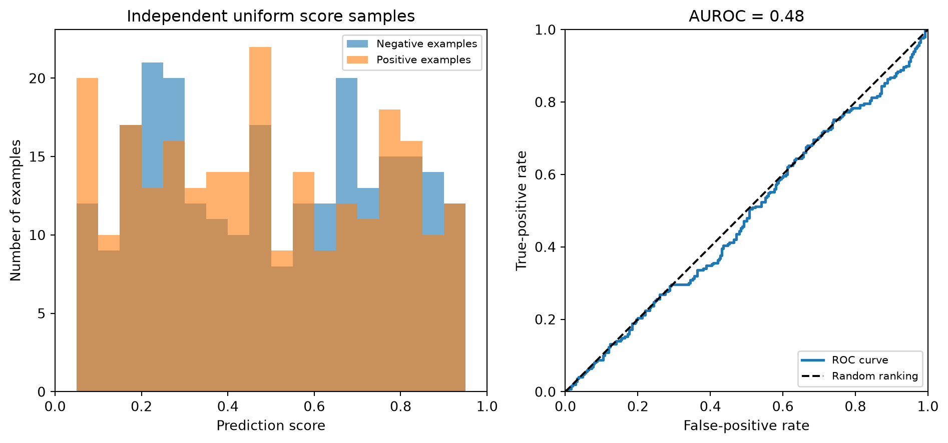
Random classifier

Two independently sampled uniform score distributions beside an ROC curve close to the random diagonal.

AUROC below 0.5

Code
reversed_negative_scores = 1 - good_negative_scores
reversed_positive_scores = 1 - good_positive_scores

fig, axes = plt.subplots(1, 2, figsize=(10, 4.5), constrained_layout=True)
plot_scores_and_roc(
    axes[0],
    axes[1],
    reversed_negative_scores,
    reversed_positive_scores,
    "Reversed score ordering",
)
plt.show()
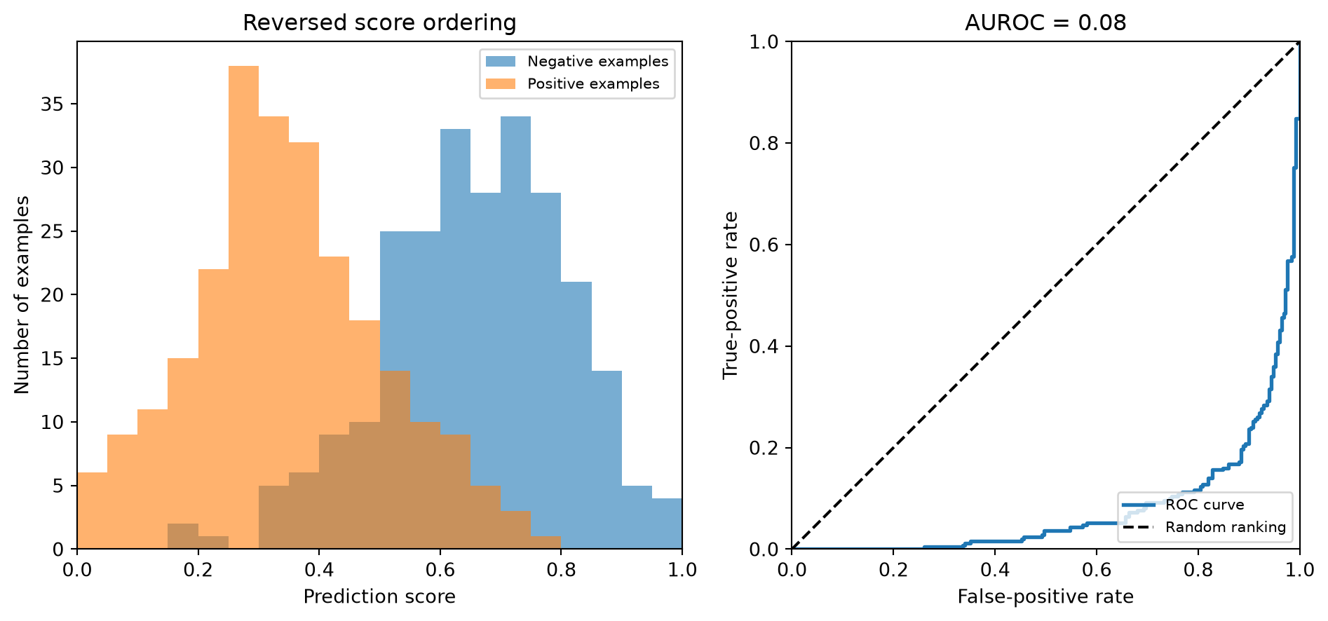
AUROC below 0.5

Positive examples receiving systematically lower scores than negative examples beside an ROC curve below the random diagonal.

ROC or precision-recall?

  • ROC uses recall and the false-positive rate, whose denominator contains all negative examples.
  • With a very rare positive class, a large number of true negatives can make the false-positive rate appear small even when many predicted positives are wrong.
  • A precision-recall curve focuses on the positive class and reveals how many positive predictions are correct.

Use the curve that matches the decision problem, and always inspect class prevalence and an operating threshold.

Constructing ROC and AUROC

Logistic Regression

  • Model:

    h_\theta(x_i) = \sigma(\theta_0 + x_i^\top\theta) = \frac{1}{1+e^{-(\theta_0+x_i^\top\theta)}}

  • Prediction:

    • Assign y_i = 0 if h_\theta(x_i) < 0.5.
    • Assign y_i = 1 if h_\theta(x_i) \geq 0.5.
  • Loss Function: cross-entropy

J(\theta) = -\frac{1}{N} \sum_{i=1}^{N} \left[ y_i \log h_\theta(x_i) + (1-y_i) \log\left(1-h_\theta(x_i)\right) \right]

Implementation: Logistic Regression

This implementation was presented in Lecture 6. It is repeated here so that the notebook contains a working model for constructing the ROC curve and computing AUROC.

Code
import numpy as np

class LogisticRegression:

    """
    Binary logistic regression trained with batch gradient descent.

    Parameters
    ----------
    learning_rate : float, default=0.1
        Step size for gradient descent.
    max_iter : int, default=1000
        Number of gradient descent iterations.
    Notes
    -----
    - This implementation expects binary labels {0, 1}.
    - The intercept (bias) term is added internally during `fit`.
    - For simplicity, there is no regularization and no early stopping.
    """

    def __init__(
        self,
        learning_rate: float = 0.1,
        max_iter: int = 1000,
    ):
        if learning_rate <= 0:
            raise ValueError("learning_rate must be positive.")
        if max_iter <= 0:
            raise ValueError("max_iter must be positive.")

        self.learning_rate = learning_rate
        self.max_iter = max_iter

        # Attributes set after fitting
        self._theta = None
        self._loss_history = None
        self._n_features = None
        self._fitted = False

    def fit(self, X: np.ndarray, y: np.ndarray) -> "LogisticRegression":
        """Fit the model parameters using gradient descent."""
        X = self._as_2d_array(X, name="X")
        y = self._as_1d_array(y, name="y")

        if X.shape[0] != y.shape[0]:
            raise ValueError(
                "X and y must contain the same number of examples."
            )
        self._check_binary_labels(y)

        n_examples, n_features = X.shape
        self._n_features = n_features
        Xb = self._add_intercept(X)

        # Zero initialization works because the objective is convex.
        self._theta = np.zeros(n_features + 1, dtype=float)
        self._loss_history = []

        for _ in range(self.max_iter):
            probabilities = self._sigmoid(Xb @ self._theta)
            gradient = (Xb.T @ (probabilities - y)) / n_examples
            self._theta -= self.learning_rate * gradient

            updated_probabilities = self._sigmoid(Xb @ self._theta)
            self._loss_history.append(
                self._bce_loss(updated_probabilities, y)
            )

        self._fitted = True
        return self

    def predict_proba(self, X: np.ndarray) -> np.ndarray:
        """Return predicted probabilities for the positive class."""
        self._ensure_fitted()
        X = self._as_2d_array(X, name="X")
        self._ensure_same_n_features(X)

        Xb = self._add_intercept(X)
        return self._sigmoid(Xb @ self._theta)

    def predict(
        self,
        X: np.ndarray,
        threshold: float = 0.5,
    ) -> np.ndarray:
        """Return class predictions using a probability threshold."""
        if not 0 <= threshold <= 1:
            raise ValueError("threshold must be between 0 and 1.")
        return (self.predict_proba(X) >= threshold).astype(int)

    @property
    def intercept_(self) -> float:
        """Return the fitted intercept."""
        self._ensure_fitted()
        return float(self._theta[0])

    @property
    def coef_(self) -> np.ndarray:
        """Return a copy of the fitted feature coefficients."""
        self._ensure_fitted()
        return self._theta[1:].copy()

    def get_loss_history(self) -> list:
        """Return a copy of the loss values collected during fitting."""
        self._ensure_fitted()
        return list(self._loss_history)

    @staticmethod
    def _sigmoid(z: np.ndarray) -> np.ndarray:
        """Compute the sigmoid without numerical overflow."""
        z = np.asarray(z, dtype=float)
        result = np.empty_like(z)
        positive = z >= 0
        result[positive] = 1.0 / (1.0 + np.exp(-z[positive]))
        exp_z = np.exp(z[~positive])
        result[~positive] = exp_z / (1.0 + exp_z)
        return result

    @staticmethod
    def _bce_loss(probabilities: np.ndarray, y: np.ndarray) -> float:
        probabilities = np.clip(probabilities, 1e-12, 1.0 - 1e-12)
        return float(
            -np.mean(
                y * np.log(probabilities)
                + (1 - y) * np.log(1 - probabilities)
            )
        )

    @staticmethod
    def _as_2d_array(X, name="X") -> np.ndarray:
        X = np.asarray(X, dtype=float)
        if X.ndim != 2:
            message = (
                f"{name} must be a 2D array of shape "
                "(n_samples, n_features)."
            )
            raise ValueError(message)
        return X

    @staticmethod
    def _as_1d_array(y, name="y") -> np.ndarray:
        y = np.asarray(y, dtype=float)
        if y.ndim != 1:
            message = f"{name} must have shape (n_samples,)."
            raise ValueError(message)
        return y

    @staticmethod
    def _check_binary_labels(y: np.ndarray) -> None:
        if not np.array_equal(np.unique(y), np.array([0.0, 1.0])):
            raise ValueError(
                "y must contain both binary labels 0 and 1."
            )

    @staticmethod
    def _add_intercept(X: np.ndarray) -> np.ndarray:
        return np.column_stack([np.ones(X.shape[0]), X])

    def _ensure_fitted(self) -> None:
        if not self._fitted or self._theta is None:
            raise RuntimeError(
                "Call fit(X, y) before using the fitted model."
            )

    def _ensure_same_n_features(self, X: np.ndarray) -> None:
        if X.shape[1] != self._n_features:
            message = (
                f"X has {X.shape[1]} features; "
                f"expected {self._n_features}."
            )
            raise ValueError(message)

Implementation: ROC

def compute_roc_curve(y_true, y_scores):
    y_true = np.asarray(y_true)
    y_scores = np.asarray(y_scores, dtype=float)
    thresholds = np.r_[np.inf, np.sort(np.unique(y_scores))[::-1]]
    tpr_list, fpr_list = [], []

    for threshold in thresholds:
        y_pred = (y_scores >= threshold).astype(int)
        tp = np.sum((y_true == 1) & (y_pred == 1))
        fn = np.sum((y_true == 1) & (y_pred == 0))
        fp = np.sum((y_true == 0) & (y_pred == 1))
        tn = np.sum((y_true == 0) & (y_pred == 0))

        tpr_list.append(tp / (tp + fn)) # true positive rate
        fpr_list.append(fp / (fp + tn)) # false positive rate

    return np.array(fpr_list), np.array(tpr_list), thresholds

Implementation: AUROC

def compute_auroc(fpr, tpr):

    return np.trapezoid(tpr, fpr)

Example: Generate Data + Predictions

Code
from sklearn.datasets import make_blobs

X, y = make_blobs(
    n_samples=1000,
    n_features=2,
    centers=2,
    cluster_std=5,
    random_state=seed,
)

X_train, X_test, y_train, y_test = train_test_split(
    X,
    y,
    test_size=0.3,
    random_state=seed,
    stratify=y,
)

model = LogisticRegression(learning_rate=0.1, max_iter=500)
model.fit(X_train, y_train)

Example: Plot

Code
# Compute predicted probabilities for the positive class on the test set
y_probs = model.predict_proba(X_test)

# Compute the ROC curve (FPR and TPR for each threshold)
fpr, tpr, thresholds = compute_roc_curve(y_test, y_probs)
auroc_value = compute_auroc(fpr, tpr)

from sklearn.metrics import roc_auc_score
sklearn_auc = roc_auc_score(y_test, y_probs)

print(f"Manual AUROC:       {auroc_value:.3f}")
print(f"scikit-learn AUROC: {sklearn_auc:.3f}")

# Plot the ROC curve
plt.figure(figsize=(8, 6))
plt.plot(
    fpr,
    tpr,
    color="blue",
    lw=2,
    label=f"ROC curve (AUROC = {auroc_value:.2f})",
)
plt.plot(
    [0, 1],
    [0, 1],
    color="gray",
    lw=1,
    linestyle="--",
    label="Random classifier",
)
plt.xlabel('False Positive Rate')
plt.ylabel('True Positive Rate')
plt.title('Receiver Operating Characteristic (ROC) Curve')
plt.legend(loc="lower right")
plt.show()
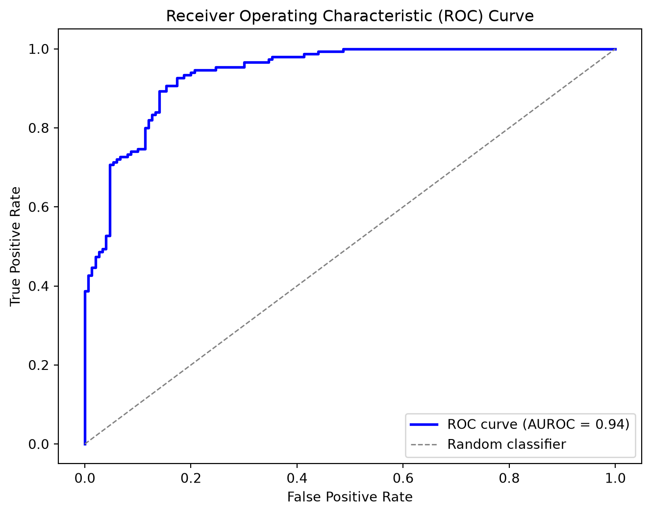
Example: Plot

Manual AUROC:       0.938
scikit-learn AUROC: 0.938

ROC curve from the lecture logistic regression implementation.

See also

Closing Material

Summary

  • Derived binary and one-vs-rest counts from confusion matrices.
  • Computed and interpreted accuracy, precision, recall, and the F_1 score, including the limitations of accuracy under class imbalance.
  • Distinguished micro averaging, which gives each prediction equal weight, from macro averaging, which gives each class equal weight.
  • Related the decision threshold to the precision-recall trade-off and to operating points on the ROC curve.
  • Interpreted AUROC as a measure of score ranking. AUROC does not assess probability calibration or select a decision threshold.

Key references

  • Sokolova and Lapalme (2009) systematically analyzes classification performance measures across binary, multiclass, and multilabel tasks.
  • Hanley and McNeil (1982) establishes the probabilistic ranking interpretation of the area under an ROC curve.
  • Davis and Goadrich (2006) explains the relationship between ROC and precision-recall curves, including the effect of skewed class distributions.

Evaluating Learning Algorithms

  • This book examines the evaluation process, with particular attention to classification algorithms (Japkowicz and Shah 2011).

  • Nathalie Japkowicz previously served as a professor at the University of Ottawa.

  • Mohak Shah earned his PhD from the University of Ottawa and has held several industry roles in AI and machine learning.

Next lecture

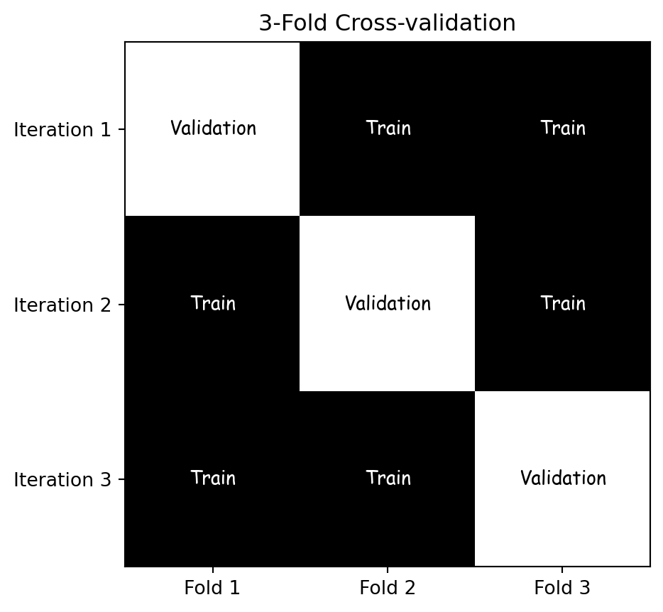
  • We will examine cross-validation and hyperparameter tuning.

References

Davis, Jesse, and Mark Goadrich. 2006. “The relationship between Precision-Recall and ROC curves.” Proceedings of the 23rd International Conference on Machine Learning - ICML ’06, 233–40. https://doi.org/10.1145/1143844.1143874.
Géron, Aurélien. 2022. Hands-on Machine Learning with Scikit-Learn, Keras, and TensorFlow. 3rd ed. O’Reilly Media, Inc.
Hanley, J A, and B J McNeil. 1982. “The meaning and use of the area under a receiver operating characteristic (ROC) curve.” Radiology 143 (1): 29–36. https://doi.org/10.1148/radiology.143.1.7063747.
Japkowicz, Nathalie, and Mohak Shah. 2011. Evaluating Learning Algorithms: A Classification Perspective. Cambridge University Press.
Knowler, William C., David J. Pettitt, Peter J. Savage, and Peter H. Bennett. 1981. “Diabetes Incidence in Pima Indians: Contributions of Obesity and Parental Diabetes.” American Journal of Epidemiology 113 2: 144–56. https://api.semanticscholar.org/CorpusID:25209675.
Russell, Stuart, and Peter Norvig. 2020. Artificial Intelligence: A Modern Approach. 4th ed. Pearson. http://aima.cs.berkeley.edu/.
Sokolova, Marina, and Guy Lapalme. 2009. “A systematic analysis of performance measures for classification tasks.” Information Processing and Management 45 (4): 427–37. https://doi.org/10.1016/j.ipm.2009.03.002.
Unceta, Irene, Paula Subı́as-Beltrán, and Oriol Pujol. 2026. “The Epistemic Debt of Generative AI.” Nature Machine Intelligence 8 (9): 1328–30. https://doi.org/10.1038/s42256-026-01294-w.

Marcel Turcotte

[email protected]

School of Electrical Engineering and Computer Science (EECS)

University of Ottawa

Appendix: 20 Newsgroups

Worked example: 20 Newsgroups

Using the 20 Newsgroups text dataset from scikit-learn.

The complete dataset contains approximately 18,000 newsgroup posts from 20 topics. This example uses four topics.

Code
from sklearn.datasets import fetch_20newsgroups
from sklearn.feature_extraction.text import TfidfVectorizer
from sklearn.linear_model import RidgeClassifier

categories = [
    "alt.atheism",
    "talk.religion.misc",
    "comp.graphics",
    "sci.space",
]

data_train = fetch_20newsgroups(
    subset="train",
    categories=categories,
    shuffle=True,
    random_state=seed,
)
data_test = fetch_20newsgroups(
    subset="test",
    categories=categories,
    shuffle=True,
    random_state=seed,
)

vectorizer = TfidfVectorizer(
    sublinear_tf=True,
    max_df=0.5,
    min_df=5,
    stop_words="english",
)
X_train = vectorizer.fit_transform(data_train.data)
X_test = vectorizer.transform(data_test.data)
y_train = data_train.target
y_test = data_test.target
target_names = data_train.target_names

clf = RidgeClassifier(tol=1e-2, solver="sparse_cg")
clf.fit(X_train, y_train)
y_pred = clf.predict(X_test)

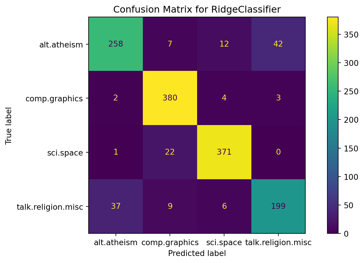
fig, ax = plt.subplots(figsize=(10, 5))
ConfusionMatrixDisplay.from_predictions(y_test, y_pred, ax=ax)
ax.xaxis.set_ticklabels(target_names)
ax.yaxis.set_ticklabels(target_names)
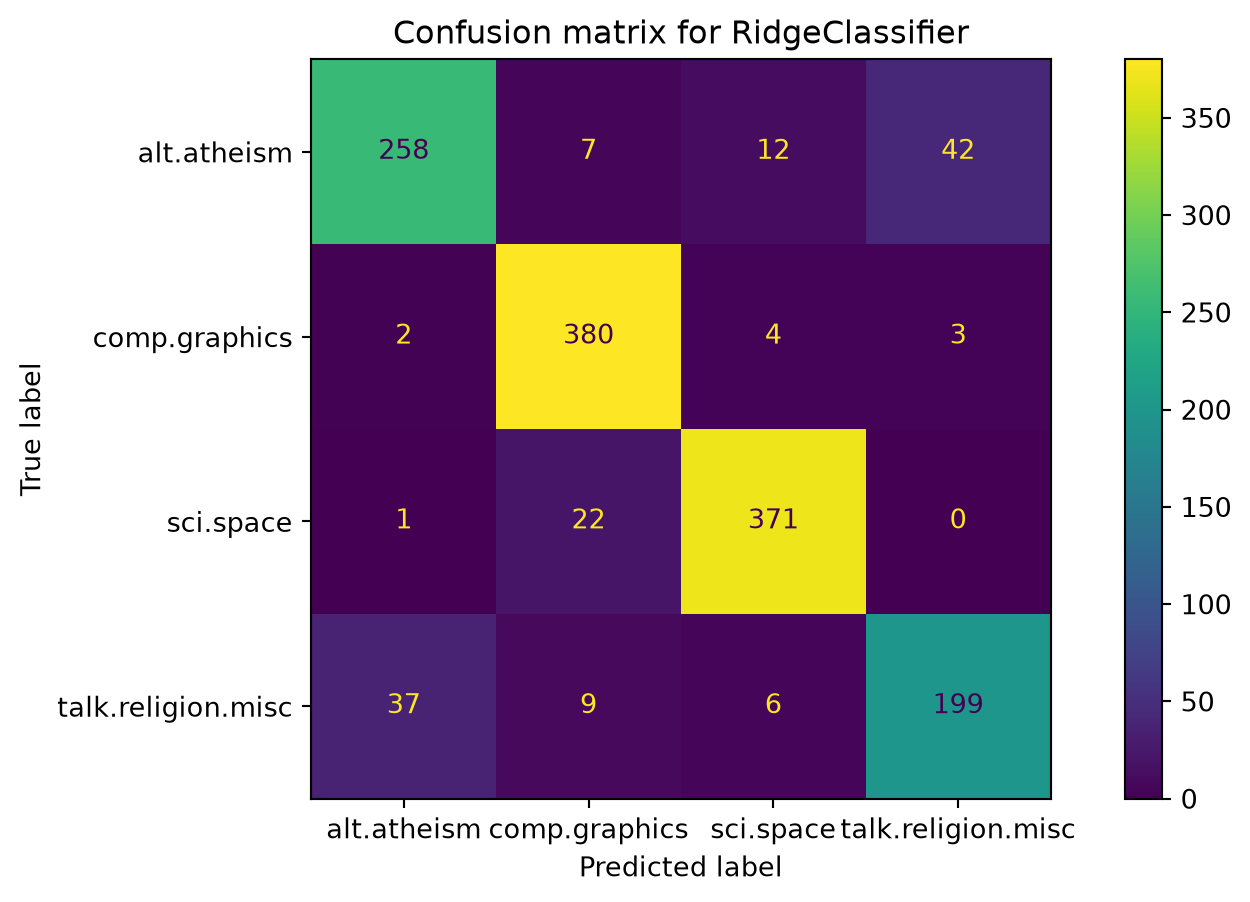
ax.set_title(f"Confusion matrix for {clf.__class__.__name__}")
plt.show()

Worked example: 20 Newsgroups

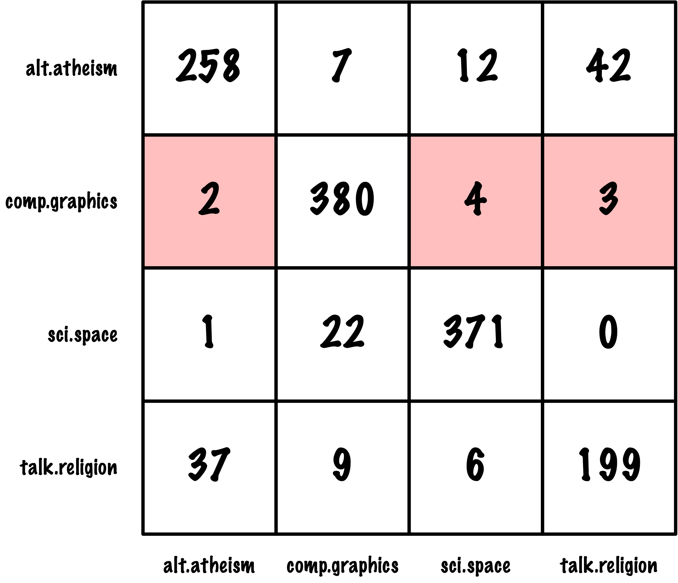
Four-class confusion matrix for selected 20 Newsgroups topics.

Confusion matrix as an array

cm = confusion_matrix(y_test, y_pred)
cm
array([[258,   7,  12,  42],
       [  2, 380,   4,   3],
       [  1,  22, 371,   0],
       [ 37,   9,   6, 199]])

One-vs-rest counts

def true_positive(cm, i):
    return cm[i, i]

def false_positive(cm, i):
    return np.sum(cm[:, i]) - cm[i, i]

def false_negative(cm, i):
    return np.sum(cm[i, :]) - cm[i, i]

def true_negative(cm, i):
    n_examples = cm.sum()
    tp = true_positive(cm, i)
    fp = false_positive(cm, i)
    fn = false_negative(cm, i)
    return n_examples - (tp + fp + fn)

Micro and macro precision

def precision_micro(cm):
    _, n_classes = cm.shape
    tp = fp = 0
    for i in range(n_classes):
        tp += true_positive(cm, i)
        fp += false_positive(cm, i)
    return tp / (tp + fp)

def precision_macro(cm):
    _, n_classes = cm.shape
    precision_sum = 0
    for i in range(n_classes):
        tp = true_positive(cm, i)
        fp = false_positive(cm, i)
        precision_sum += tp / (tp + fp)
    return precision_sum / n_classes

print(f"Micro precision: {precision_micro(cm):.3f}")
print(f"Macro precision: {precision_macro(cm):.3f}")
Micro precision: 0.893
Macro precision: 0.884

Micro-average precision

\frac{(258+380+371+199)}{(258+380+371+199)+(40+38+22+45)} where

  • 40 = 2 + 1 + 37
  • 38 = 7 + 22 + 9
  • 22 = 12 + 4 + 6
  • 45 = 42 + 3 + 0

Macro-average precision

  • \mathrm{Precision}_0 = \frac{258}{258+(2+1+37)} = 0.8657718121
  • \mathrm{Precision}_1 = \frac{380}{380+(7+22+9)} = 0.9090909091
  • \mathrm{Precision}_2 = \frac{371}{371+(12+4+6)} = 0.9440203562
  • \mathrm{Precision}_3 = \frac{199}{199+(42+3+0)} = 0.8155737705

\mathrm{Precision}_{\mathrm{macro}} = \frac{0.8657718121 + 0.9090909091 + 0.9440203562 + 0.8155737705}{4}

Micro and macro recall

def recall_micro(cm):
    _, n_classes = cm.shape
    tp = fn = 0
    for i in range(n_classes):
        tp += true_positive(cm, i)
        fn += false_negative(cm, i)
    return tp / (tp + fn)

def recall_macro(cm):
    _, n_classes = cm.shape
    recall_sum = 0
    for i in range(n_classes):
        tp = true_positive(cm, i)
        fn = false_negative(cm, i)
        recall_sum += tp / (tp + fn)
    return recall_sum / n_classes

print(f"Micro recall: {recall_micro(cm):.3f}")
print(f"Macro recall: {recall_macro(cm):.3f}")
Micro recall: 0.893
Macro recall: 0.880

Appendix: Comparing Classifier Scores

OpenML dataset

OpenML is an open platform for sharing datasets, algorithms, and experiments that support reproducible machine learning.

diabetes = fetch_openml(name='diabetes', version=1)
print(diabetes.DESCR)

OpenML dataset

Author: Vincent Sigillito

Source: Obtained from UCI

Please cite: UCI citation policy

  1. Title: Pima Indians Diabetes Database

  2. Sources:

    1. Original owners: National Institute of Diabetes and Digestive and Kidney Diseases
    2. Donor of database: Vincent Sigillito ([email protected]) Research Center, RMI Group Leader Applied Physics Laboratory The Johns Hopkins University Johns Hopkins Road Laurel, MD 20707 (301) 953-6231
    3. Date received: 9 May 1990
  3. Past Usage:

    1. Smith,J.W., Everhart,J.E., Dickson,W.C., Knowler,W.C., & Johannes,R.S. (1988). Using the ADAP learning algorithm to forecast the onset of diabetes mellitus. In {it Proceedings of the Symposium on Computer Applications and Medical Care} (pp. 261–265). IEEE Computer Society Press.

      The diagnostic, binary-valued variable investigated is whether the patient shows signs of diabetes according to World Health Organization criteria (i.e., if the 2 hour post-load plasma glucose was at least 200 mg/dl at any survey examination or if found during routine medical care). The population lives near Phoenix, Arizona, USA.

      Results: Their ADAP algorithm makes a real-valued prediction between 0 and 1. This was transformed into a binary decision using a cutoff of 0.448. Using 576 training instances, the sensitivity and specificity of their algorithm was 76% on the remaining 192 instances.

  4. Relevant Information: Several constraints were placed on the selection of these instances from a larger database. In particular, all patients here are females at least 21 years old of Pima Indian heritage. ADAP is an adaptive learning routine that generates and executes digital analogs of perceptron-like devices. It is a unique algorithm; see the paper for details.

  5. Number of Instances: 768

  6. Number of Attributes: 8 plus class

  7. For Each Attribute: (all numeric-valued)

    1. Number of times pregnant
    2. Plasma glucose concentration a 2 hours in an oral glucose tolerance test
    3. Diastolic blood pressure (mm Hg)
    4. Triceps skin fold thickness (mm)
    5. 2-Hour serum insulin (mu U/ml)
    6. Body mass index (weight in kg/(height in m)^2)
    7. Diabetes pedigree function
    8. Age (years)
    9. Class variable (0 or 1)
  8. Missing Attribute Values: None

  9. Class Distribution: (class value 1 is interpreted as “tested positive for diabetes”)

    Class Value Number of instances 0 500 1 268

  10. Brief statistical analysis:

    Attribute number: Mean: Standard Deviation:

    1.                 3.8     3.4
    2.               120.9    32.0
    3.                69.1    19.4
    4.                20.5    16.0
    5.                79.8   115.2
    6.                32.0     7.9
    7.                 0.5     0.3
    8.                33.2    11.8

Relabeled values in attribute ‘class’ From: 0 To: tested_negative
From: 1 To: tested_positive

Downloaded from openml.org.

Pima Indians Diabetes Dataset

# Load the Pima Indians Diabetes dataset
pima = fetch_openml(data_id=37, as_frame=True)

# Extract the features and target
X = pima.data
y = pima.target

# Encode the two target labels as 0 and 1
y = y.map({'tested_negative': 0, 'tested_positive': 1})

# Split the dataset
X_train, X_test, y_train, y_test = train_test_split(
    X,
    y,
    test_size=0.3,
    random_state=seed,
    stratify=y,
)

Comparing Multiple Classifiers

from sklearn.linear_model import LogisticRegression
from sklearn.neighbors import KNeighborsClassifier
from sklearn.tree import DecisionTreeClassifier
from sklearn.ensemble import RandomForestClassifier

Comparing Multiple Classifiers

Code
scaler = StandardScaler()
X_train_scaled = scaler.fit_transform(X_train)
X_test_scaled = scaler.transform(X_test)

lr = LogisticRegression(max_iter=1000)
lr.fit(X_train_scaled, y_train)

knn = KNeighborsClassifier()
knn.fit(X_train_scaled, y_train)

dt = DecisionTreeClassifier(random_state=seed)
dt.fit(X_train, y_train)

rf = RandomForestClassifier(random_state=seed)
rf.fit(X_train, y_train)

ROC curves and AUROC

Code
from sklearn.metrics import roc_auc_score

y_pred_prob_lr = lr.predict_proba(X_test_scaled)[:, 1]
y_pred_prob_knn = knn.predict_proba(X_test_scaled)[:, 1]
y_pred_prob_dt = dt.predict_proba(X_test)[:, 1]
y_pred_prob_rf = rf.predict_proba(X_test)[:, 1]

# Compute ROC curves
fpr_lr, tpr_lr, _ = roc_curve(y_test, y_pred_prob_lr)
fpr_knn, tpr_knn, _ = roc_curve(y_test, y_pred_prob_knn)
fpr_dt, tpr_dt, _ = roc_curve(y_test, y_pred_prob_dt)
fpr_rf, tpr_rf, _ = roc_curve(y_test, y_pred_prob_rf)

# Compute AUROC scores
auc_lr = roc_auc_score(y_test, y_pred_prob_lr)
auc_knn = roc_auc_score(y_test, y_pred_prob_knn)
auc_dt = roc_auc_score(y_test, y_pred_prob_dt)
auc_rf = roc_auc_score(y_test, y_pred_prob_rf)

# Plot ROC curves
plt.figure(figsize=(5, 5))
plt.plot(
    fpr_lr,
    tpr_lr,
    color="blue",
    label=f"Logistic Regression (AUROC = {auc_lr:.2f})",
)
plt.plot(
    fpr_knn,
    tpr_knn,
    color="green",
    label=f"K-Nearest Neighbors (AUROC = {auc_knn:.2f})",
)
plt.plot(
    fpr_dt,
    tpr_dt,
    color="orange",
    label=f"Decision Tree (AUROC = {auc_dt:.2f})",
)
plt.plot(
    fpr_rf,
    tpr_rf,
    color="purple",
    label=f"Random Forest (AUROC = {auc_rf:.2f})",
)
plt.plot([0, 1], [0, 1], color="red", linestyle="--")
plt.xlim([0.0, 1.0])
plt.ylim([0.0, 1.05])
plt.xlabel("False Positive Rate")
plt.ylabel("True Positive Rate")
plt.title("ROC curves on the Pima diabetes test set")
plt.legend(loc="lower right")
plt.show()
ROC curves for four classifiers on the Pima diabetes test set.