Model Evaluation and Hyperparameter Tuning

CSI 4106 - Fall 2026

Marcel Turcotte

Version: Sep 25, 2026 08:51

Preamble

Message of the Day

Note

A comedy writer explores the implications of artificial intelligence through a collaborative poetry book project with a childhood friend working at OpenAI. This personal journey examines the tension between professional ambitions in tech and the preservation of human creativity as the prospect of future superintelligence looms over their long-standing friendship.

Daniel Kokotajlo shared on X a personal statement about AI risk written by Daniel Selsam, the OpenAI employee featured in the video.

An OpenAI Engineer and His Friends Debate the Future, The New Yorker Documentary, 2026-09-23.

Learning Objectives

• Distinguish the roles of training, validation, and test data in model development and final evaluation.
• Explain how k-fold cross-validation trains a new model in each iteration and interpret the mean and standard deviation of its related fold scores.
• Prevent data leakage by fitting preprocessing within each fold and applying stored transformations to validation and test examples.
• Distinguish learned model parameters from hyperparameters and explain why interacting hyperparameters should be evaluated jointly.
• Apply GridSearchCV to tune multiple pipelines using a consistent metric and explain when randomized search is useful.
• Compare tuned model families, refit the selected pipeline on all training data, and evaluate it once on the untouched test set.

Introduction

Dataset: OpenML

www.openml.org

OpenML is an open platform for sharing datasets, algorithms, and experiments - to learn how to learn better, together.

import numpy as np
seed = 42

from sklearn.datasets import fetch_openml

diabetes = fetch_openml(name='diabetes', version=1)
print(diabetes.DESCR)

The Pima diabetes dataset contains 768 examples and eight numerical attributes. It is compact enough to make repeated cross-validation practical during class. Its restricted study population, age, and data-quality limitations prevent the results from supporting broad medical conclusions.

Dataset: OpenML

Author: Vincent Sigillito

Source: Obtained from UCI

Please cite: UCI citation policy

1. Title: Pima Indians Diabetes Database

2. Sources:

   1. Original owners: National Institute of Diabetes and Digestive and Kidney Diseases
   2. Donor of database: Vincent Sigillito ([email protected]) Research Center, RMI Group Leader Applied Physics Laboratory The Johns Hopkins University Johns Hopkins Road Laurel, MD 20707 (301) 953-6231
   3. Date received: 9 May 1990

3. Past Usage:

   1. Smith,_J.W., Everhart,_J.E., Dickson,_W.C., Knowler,_W.C., & Johannes,_R.S. (1988). Using the ADAP learning algorithm to forecast the onset of diabetes mellitus. In {it Proceedings of the Symposium on Computer Applications and Medical Care} (pp. 261–265). IEEE Computer Society Press.

      The diagnostic, binary-valued variable investigated is whether the patient shows signs of diabetes according to World Health Organization criteria (i.e., if the 2 hour post-load plasma glucose was at least 200 mg/dl at any survey examination or if found during routine medical care). The population lives near Phoenix, Arizona, USA.

      Results: Their ADAP algorithm makes a real-valued prediction between 0 and 1. This was transformed into a binary decision using a cutoff of 0.448. Using 576 training instances, the sensitivity and specificity of their algorithm was 76% on the remaining 192 instances.

4. Relevant Information: Several constraints were placed on the selection of these instances from a larger database. In particular, all patients here are females at least 21 years old of Pima Indian heritage. ADAP is an adaptive learning routine that generates and executes digital analogs of perceptron-like devices. It is a unique algorithm; see the paper for details.

5. Number of Instances: 768

6. Number of Attributes: 8 plus class

7. For Each Attribute: (all numeric-valued)

   1. Number of times pregnant
   2. Plasma glucose concentration a 2 hours in an oral glucose tolerance test
   3. Diastolic blood pressure (mm Hg)
   4. Triceps skin fold thickness (mm)
   5. 2-Hour serum insulin (mu U/ml)
   6. Body mass index (weight in kg/(height in m)^2)
   7. Diabetes pedigree function
   8. Age (years)
   9. Class variable (0 or 1)

8. Missing Attribute Values: None

9. Class Distribution: (class value 1 is interpreted as “tested positive for diabetes”)

   Class Value Number of instances 0 500 1 268

10. Brief statistical analysis:

    Attribute number: Mean: Standard Deviation:

    1.                 3.8     3.4

    2.               120.9    32.0

    3.                69.1    19.4

    4.                20.5    16.0

    5.                79.8   115.2

    6.                32.0     7.9

    7.                 0.5     0.3

    8.                33.2    11.8

Relabeled values in attribute ‘class’ From: 0 To: tested_negative
From: 1 To: tested_positive

Downloaded from openml.org.

Dataset: return_X_y

fetch_openml returns a Bunch by default, or X and y when return_X_y=True.

X, y = fetch_openml(name='diabetes', version=1, return_X_y=True)

The positive class is less frequent, but both classes have enough examples for stratified cross-validation.

print(y.value_counts())

class
tested_negative    500
tested_positive    268
Name: count, dtype: int64

Convert the target labels to 0 and 1:

y = y.map({'tested_negative': 0, 'tested_positive': 1})

The dataset contains 500 negative and 268 positive examples, corresponding to an approximately 65:35 class distribution. This moderate imbalance does not automatically justify resampling or class weighting. Stratification approximately preserves these proportions in the training, validation, and test partitions, but it does not correct the imbalance itself.

Any additional intervention should depend on the evaluation objective and the relative consequences of false positives and false negatives. Methods for handling class imbalance will be examined later. AUROC remains useful for comparing score rankings here, while the final classification report reveals differences in class-specific performance.

Missing measurements

Following the convention used by the corrected PimaIndiansDiabetes2 version of this dataset, zero values in five clinical measurements are treated as missing. Zero remains valid for the number of pregnancies.

missing_value_columns = ["plas", "pres", "skin", "insu", "mass"]

X = X.copy()
X[missing_value_columns] = X[missing_value_columns].replace(0, np.nan)

X[missing_value_columns].isna().sum()

plas      5
pres     35
skin    227
insu    374
mass     11
dtype: int64

The OpenML metadata reports no missing attribute values. However, the PimaIndiansDiabetes2 documentation describes these zeros as physical impossibilities and treats them as missing. This is therefore a documented preprocessing convention rather than a rule supplied by OpenML.

The replacement does not estimate any value from the dataset. Median imputation will be learned later from each training fold, which prevents information from a validation fold or the test set from influencing the transformation.

Cross-validation

Training and test sets

This division is often called the holdout method.

• Common starting point: Allocate 80% of the data to training and reserve 20% for testing.

• Training set: Used to fit models and make model-building choices.

• Test set: An independent subset used once for the final evaluation.

Common Training and Testing Ratios

1. 80:20 split:
   • Training Set: 80% of the data
   • Test Set: 20% of the data
   • This is a widely used default split that provides a balance between having enough data to train the model and enough data to evaluate its performance.
2. 90:10 split:
   • Training Set: 90% of the data
   • Test Set: 10% of the data
   • This split may be appropriate for a large dataset when 10% still provides enough examples for a useful evaluation.

Considerations for Choosing the Split Ratio

1. Dataset Size:
   • For large datasets, a smaller proportion can be reserved for testing (e.g., 90:10) when it still provides enough test examples for a useful evaluation.
2. Model Complexity:
   • Complex models with many parameters may require more training data to avoid overfitting, suggesting a larger training set.
3. Validation Data:
   • Cross-validation can reuse the training data for validation. A separate validation set may be preferable when computational cost or the data structure makes cross-validation impractical.
4. Imbalanced Datasets:
   • Both splits must contain enough examples from each class. Stratified sampling approximately preserves the class proportions in the training and test sets.

Training and test sets

Training error: The prediction error measured on examples used to fit the model.

• Model fitting generally seeks to reduce training loss or error.
• A low training error does not guarantee a low generalization error.

Training and test sets

Generalization error: The expected prediction error on new examples drawn under similar conditions.

It cannot be observed directly. Validation and test scores provide estimates from finite samples.

Training and test sets

Underfitting:

• High training error
• Model is too simple to capture underlying patterns
• Poor performance on both training and new data

Overfitting:

• Low training error, but high generalization error
• Model captures noise or irrelevant patterns
• Poor performance on new, unseen data

Definition

Cross-validation estimates how well a model-building procedure will perform on unseen examples.

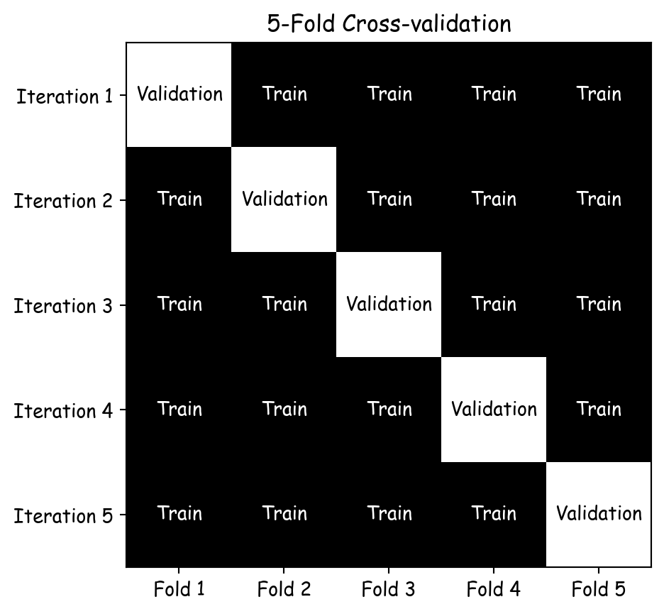
It repeatedly partitions the training data, trains a new classifier on some folds, and evaluates that classifier on the remaining fold. The test set remains untouched.

k-fold cross-validation

1. Divide the training data into k approximately equal parts (folds).
2. Repeat k times:
   • Start with a new, unfitted classifier.
   • Train it on k-1 folds.
   • Evaluate it on the remaining validation fold.
3. Aggregation: Summarize the k scores produced by the k separately trained classifiers.

Each iteration produces a distinct fitted classifier. Learned parameters are not carried from one iteration to the next. Cross-validation therefore evaluates a model-building procedure rather than one persistent classifier.

The k scores describe performance on different validation folds. Their average depends less on one arbitrary split than a single validation score.

The fitted classifiers nevertheless share most of their training examples. With five folds, for example, any two classifiers share three complete folds: 60% of the full training dataset, or 75% of the examples used to fit either classifier. Although their validation folds differ, the fitted classifiers and their scores are therefore related rather than independent.

The standard deviation is a descriptive measure of variation across these particular folds. It is not a standard error, and dividing it by \sqrt{k} does not produce a valid confidence interval. A small value does not by itself establish that the learning procedure is stable, while a large value may reflect unusually difficult or compositionally different validation folds.

After model and hyperparameter selection, a final classifier is fitted on the complete training set.

import matplotlib.pyplot as plt

def plot_k_fold_cross_validation(k):
    fig, ax = plt.subplots()

    matrix = np.ones((k, k))
    np.fill_diagonal(matrix, 0)

    ax.imshow(matrix, cmap='binary', interpolation='none')

    for i in range(k):
        for j in range(k):
            label = 'Validation' if i == j else 'Train'
            color = "black" if i == j else "white"
            ax.text(j, i, label, ha="center", va="center", color=color)

    ax.set_xticks(np.arange(k))
    ax.set_yticks(np.arange(k))
    ax.set_xticklabels([f"Fold {i+1}" for i in range(k)])
    ax.set_yticklabels([f"Iteration {i+1}" for i in range(k)])
    plt.title(f'{k}-Fold Cross-validation')

    ax.grid(False)
    plt.show()

Common choices for the value of k are 5 and 10.

5-fold cross-validation

plot_k_fold_cross_validation(5)

Each row represents one iteration. Every fold serves once as the validation fold and four times as part of the training data. These folds come only from the training portion of the original dataset. The held-out test examples do not participate in this process.

With each iteration, 4/5 of the training data is used for fitting and 1/5 for validation.

Evaluation across validation folds

• During model selection, cross-validation averages scores across several validation folds rather than relying on one validation partition.
• One score per fold reveals sensitivity to the particular validation examples.
• The mean and standard deviation summarize the fold scores, but the scores are not independent.

The final test set is also one finite sample, and its score depends on which examples it contains. Its purpose is not to remove sampling variability. Its purpose is to provide a final evaluation using examples that did not influence model or hyperparameter selection.

Repeatedly consulting alternative test splits would allow their results to influence model development and would gradually turn them into validation data. When uncertainty in the final score matters, it should be quantified using an appropriate confidence interval or bootstrap procedure applied to the untouched test predictions. Nested cross-validation or a genuinely independent external dataset provides another option when a single holdout set is inadequate.

Estimating generalization

• Cross-validation estimates performance on unseen examples drawn under similar conditions.
• It does not improve generalization by itself. It helps compare model-building choices using only the training data.
• The untouched test set provides the final evaluation after those choices have been made.

Efficient use of data

• Cross-validation is particularly useful when data is limited.
• Across the k iterations, each training example appears once in a validation fold and k-1 times in a fitting fold.
• After model selection, the chosen procedure can be refitted on the complete training set.

Examples need not be equally informative to the learning algorithm. The composition of each fitting and validation fold can therefore affect its score.

Hyperparameter tuning

• Cross-validation compares candidate hyperparameter settings using the same folds and evaluation metric.
• The selected setting has the best estimated performance among the candidates that were evaluated.

The highest cross-validation score is used to select the hyperparameter setting, so it can be somewhat optimistic. The final test evaluation estimates the performance of the complete selection procedure on data that did not influence that choice.

Challenges

• Computational cost: Requires repeated model fitting.
  • Leave-one-out (LOO) is the extreme case where ( k = N ).
• Class imbalance: Random folds may not adequately represent minority classes.
  • Use stratified cross-validation to approximately maintain class proportions.
• Implementation complexity: Manual implementations are error-prone, especially for nested cross-validation, bootstrap resampling, or integration into larger pipelines.

Leave-one-out cross-validation fits the model once for every example. Its training sets differ by only one example, which can produce a high-variance estimate for some learning procedures and makes it computationally expensive. Five- or ten-fold cross-validation is usually a more practical default.

Stratified cross-validation approximately preserves the class distribution in every fold so that each class is represented in the fitting and validation partitions.

Ordinary random folds also assume that examples can be exchanged without changing the problem. Repeated measurements from the same person require group-aware folds, and predictions about the future require a time-aware split.

Hyperparameter tuning

Workflow

This workflow distinguishes three uses of data: training, validation, and test. The validation folds support model selection, while the test set remains outside that process.

Attribution: Cross-validation: evaluating estimator performance

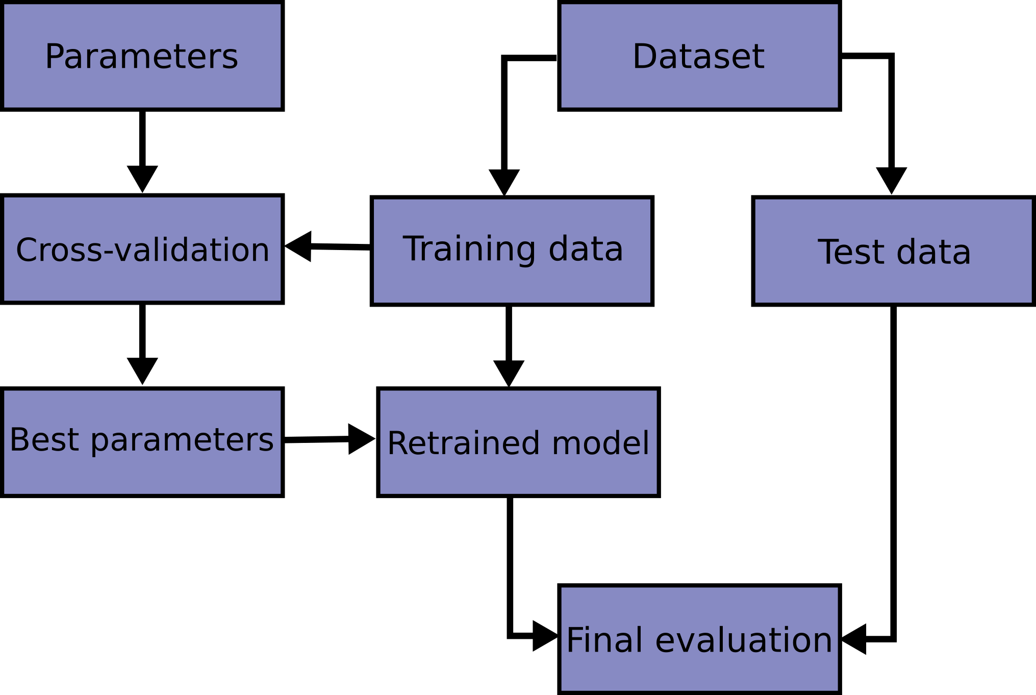
Workflow: implementation

from sklearn.model_selection import (
    StratifiedKFold,
    cross_val_score,
    train_test_split,
)

X_train, X_test, y_train, y_test = train_test_split(
    X,
    y,
    test_size=0.2,
    random_state=seed,
    stratify=y,
)

cv = StratifiedKFold(n_splits=5, shuffle=True, random_state=seed)
selection_metric = "roc_auc"

The test set is separated before cross-validation and hyperparameter tuning. Stratification preserves approximately the same class proportions in both partitions. The explicit cross-validation object makes the folds reproducible and ensures that every model uses the same validation splits.

AUROC is the selection metric throughout this example. Changing the metric could change which hyperparameters and model are selected.

Data leakage during cross-validation

Data leakage occurs when information from a validation fold influences the procedure fitted on the remaining folds.

# Incorrect: the scaler sees every future validation fold

scaler = StandardScaler()
X_train_scaled = scaler.fit_transform(X_train)

scores = cross_val_score(
    KNeighborsClassifier(),
    X_train_scaled,
    y_train,
    cv=cv,
)

The validation examples influence the means and scales used to evaluate them.

Keeping the final test set untouched does not make this cross-validation procedure valid. The call to fit_transform occurs before the folds are created, so the scaler computes each feature’s mean and scale from all of X_train. Every validation fold therefore contributes information to its own preprocessing.

Applying fit_transform to the complete dataset X before creating the train–test split would be even more serious. The fitted transformation would then contain information from the test examples. Consequently, the test set would no longer provide an independent evaluation of the complete modelling procedure.

This is leakage even though scaling does not use the target labels. The same problem applies to imputation, feature selection, principal component analysis, resampling, and any other data-dependent operation performed before cross-validation.

A pipeline prevents this form of leakage only for operations placed inside the pipeline. It cannot correct target leakage, an inappropriate time split, or repeated observations from one subject appearing in both fitting and validation folds.

fit_transform and transform

• fit(X) learns information from X.
• fit_transform(X) learns that information and applies the transformation to the same examples.
• transform(X) applies the stored information without recomputing it.

scaler = StandardScaler()

X_fitting_folds_scaled = scaler.fit_transform(X_fitting_folds)
X_validation_fold_scaled = scaler.transform(X_validation_fold)

Validation, test, and future examples receive transform, never fit or fit_transform.

For StandardScaler, fit learns and stores attributes such as mean_ and scale_. For SimpleImputer, it stores the replacement value for each feature in statistics_. Conceptually, fit_transform(X) performs fit(X) followed by transform(X) on the same fitting examples.

Data leakage is a serious methodological problem. It has been the focus of many sessions at machine learning conferences and workshops because seemingly harmless preprocessing performed at the wrong stage can invalidate an evaluation.

The fitted transformer retains this state in memory. A fitted pipeline retains the state of every preprocessing step together with the classifier’s learned parameters. Calling predict or predict_proba on new examples automatically applies each stored transformation before invoking the classifier.

Retaining state in memory is not the same as saving it permanently. Deployment requires explicitly serializing the complete fitted pipeline so that future examples receive the same transformations. Lecture 10 examines those engineering details.

Preprocessing within each fold

For every fold, cross-validation creates and fits a new pipeline.

Pipeline step	Fitting folds	Validation fold
Imputer	fit_transform	transform
Scaler	fit_transform	transform
Classifier	fit	predict_proba / decision_function

Learned medians, means, and scales are not carried into the next fold.

For each iteration, scikit-learn clones the unfitted pipeline. Calling fit on that pipeline fits each transformer on the fitting folds and passes the transformed output to the next step. The classifier is then fitted on the fully transformed fitting examples.

When the validation fold is scored, the pipeline calls only transform on the imputer and scaler. Their stored statistics come exclusively from the fitting folds. The temporary fitted pipeline is discarded after that fold has been evaluated, and the next iteration begins with a new unfitted clone.

GridSearchCV repeats this complete process for every hyperparameter combination. After selecting a configuration, it refits that complete pipeline on all the training data and retains it as best_estimator_. The untouched test examples then receive only the transformations stored in that final fitted pipeline.

Preprocessing pipelines

from sklearn.impute import SimpleImputer
from sklearn.linear_model import LogisticRegression
from sklearn.neighbors import KNeighborsClassifier
from sklearn.pipeline import Pipeline
from sklearn.preprocessing import StandardScaler
from sklearn.tree import DecisionTreeClassifier

tree_pipeline = Pipeline([
    ("imputer", SimpleImputer(strategy="median")),
    ("model", DecisionTreeClassifier(random_state=seed)),
])

knn_pipeline = Pipeline([
    ("imputer", SimpleImputer(strategy="median")),
    ("scaler", StandardScaler()),
    ("model", KNeighborsClassifier()),
])

logistic_pipeline = Pipeline([
    ("imputer", SimpleImputer(strategy="median")),
    ("scaler", StandardScaler()),
    ("model", LogisticRegression(
        solver="saga",
        max_iter=3000,
        random_state=seed,
    )),
])

The imputer belongs inside each pipeline so that it learns its medians from a fitting fold and applies them to the corresponding validation fold. KNN and logistic regression also use standardized features because their calculations depend on distances or coefficient optimization. Decision trees split one feature at a time and do not require scaling.

The fixed value of max_iter gives the logistic-regression optimizer enough iterations to converge. It is an implementation control, not a model-complexity setting to be tuned for predictive performance.

cross_val_score

knn_scores = cross_val_score(
    knn_pipeline,
    X_train,
    y_train,
    cv=cv,
    scoring=selection_metric,
)

print("Scores:", knn_scores)
print(f"Mean AUROC: {knn_scores.mean():.3f}")
print(f"Standard deviation: {knn_scores.std():.3f}")

Scores: [0.81133721 0.76061047 0.84447674 0.74883721 0.75639881]
Mean AUROC: 0.784
Standard deviation: 0.037

Each score comes from a different validation fold. The mean summarizes the five validation results. The standard deviation describes their variation, but it is not a confidence interval because the fitted models share many training examples.

Here, cross_val_score receives the complete KNN pipeline. It therefore refits the imputer and scaler inside every fold before fitting the classifier. Passing an array that had already been imputed or standardized using all of X_train would bypass this protection.

sklearn.model_selection.cross_val_score. See also cross_validate.

Parameters and hyperparameters

Model parameters are learned from the training data.

Hyperparameters are chosen before each fit and control the model structure or learning process.

Examples of hyperparameters include a tree’s max_depth, KNN’s n_neighbors, and logistic regression’s C. Hyperparameter tuning uses validation performance to choose among candidates. The learning algorithm fits new model parameters for every candidate and every cross-validation fold.

Hyperparameters: decision tree

• criterion: chooses how the quality of a split is measured: gini, entropy, or log_loss.
• max_depth: limits the maximum depth of the tree.

See: DecisionTreeClassifier

Hyperparameters: logistic regression

• C: inverse regularization strength. Smaller values apply stronger regularization.
• l1_ratio: selects the balance between L2 and L1 regularization when the saga solver is used.

See: LogisticRegression.

Hyperparameters: KNN

• n_neighbors: number of neighbours used to make a prediction.
• weights: gives neighbours equal influence (uniform) or greater influence when they are closer (distance).

See: KNeighborsClassifier

Experiment: n_neighbors

neighbor_scores = {}
neighbor_values = [1, 3, 5, 7, 9, 11, 15, 21, 31]

for value in neighbor_values:
    candidate = knn_pipeline.set_params(
        model__n_neighbors=value,
        model__weights="uniform",
    )
    scores = cross_val_score(
        candidate,
        X_train,
        y_train,
        cv=cv,
        scoring=selection_metric,
    )
    neighbor_scores[value] = scores.mean()
    print(f"n_neighbors={value:2d}: {scores.mean():.3f}")

best_n_neighbors = max(neighbor_scores, key=neighbor_scores.get)
print("Best n_neighbors:", best_n_neighbors)

Experiment: n_neighbors

n_neighbors= 1: 0.664
n_neighbors= 3: 0.764
n_neighbors= 5: 0.784
n_neighbors= 7: 0.798
n_neighbors= 9: 0.815
n_neighbors=11: 0.822
n_neighbors=15: 0.832
n_neighbors=21: 0.831
n_neighbors=31: 0.831
Best n_neighbors: 15

Experiment: weights

weight_scores = {}

for value in ["uniform", "distance"]:
    candidate = knn_pipeline.set_params(
        model__n_neighbors=best_n_neighbors,
        model__weights=value,
    )
    scores = cross_val_score(
        candidate,
        X_train,
        y_train,
        cv=cv,
        scoring=selection_metric,
    )
    weight_scores[value] = scores.mean()
    print(f"weights={value:8s}: {scores.mean():.3f}")

weights=uniform : 0.832
weights=distance: 0.833

The first loop chooses n_neighbors while fixing weights="uniform". The second loop then fixes that chosen number of neighbours while varying weights. This sequential procedure never revisits n_neighbors after the weighting rule changes, so it can miss the best pair of values.

Evaluating the Cartesian product of the two candidate sets addresses that limitation. The code is straightforward to write with nested loops, which makes grid search conceptually simple rather than a black box.

Hyperparameter tuning: grid search

• Several hyperparameters may need to be considered together.

• Manual exploration of their combinations is tedious and error-prone.

• Grid search evaluates a predefined set of combinations systematically:

  1. Enumerate the Cartesian product of the candidate values.

  2. Evaluate each combination using the same cross-validation folds and metric.

The manual loops demonstrate that grid search can be implemented independently. A standardized implementation adds several practical benefits:

• It enumerates parameter combinations consistently.
• It applies every pipeline step separately within each fitting fold.
• It records fold-level and aggregate results in cv_results_.
• It exposes best_params_, best_score_, and a refitted best_estimator_.
• It supports several metrics, parallel execution, and explicit error reporting.
• It reduces indexing and bookkeeping mistakes and makes the experiment easier to reproduce.

The utility does not decide which metric, folds, models, or parameter values are appropriate. Those choices remain part of the experimental design.

GridSearchCV: decision tree

from sklearn.model_selection import GridSearchCV

tree_param_grid = {
    "model__max_depth": [2, 3, 4, 5, 6, None],
    "model__criterion": ["gini", "entropy", "log_loss"],
}

tree_search = GridSearchCV(
    tree_pipeline,
    tree_param_grid,
    cv=cv,
    scoring=selection_metric,
)
tree_search.fit(X_train, y_train)

(tree_search.best_params_, tree_search.best_score_)

({'model__criterion': 'gini', 'model__max_depth': 4},
 np.float64(0.7881160022148395))

GridSearchCV: KNN

knn_param_grid = {
    "model__n_neighbors": neighbor_values,
    "model__weights": ["uniform", "distance"],
}

knn_search = GridSearchCV(
    knn_pipeline,
    knn_param_grid,
    cv=cv,
    scoring=selection_metric,
)
knn_search.fit(X_train, y_train)

(knn_search.best_params_, knn_search.best_score_)

({'model__n_neighbors': 21, 'model__weights': 'distance'},
 np.float64(0.8336620985603543))

The double underscore separates the pipeline-step name from the estimator parameter. Grid search now evaluates every combination of n_neighbors and weights, rather than committing to one value before exploring the other.

With the current folds, sequential tuning selects 15 neighbours before comparing the weighting rules. The joint grid instead selects 21 neighbours with distance weighting. The difference provides a concrete example of an interaction between hyperparameters.

GridSearchCV: logistic regression

logistic_param_grid = {
    "model__C": [0.01, 0.1, 1, 10, 100],
    "model__l1_ratio": [0.0, 1.0],
}

logistic_search = GridSearchCV(
    logistic_pipeline,
    logistic_param_grid,
    cv=cv,
    scoring=selection_metric,
)
logistic_search.fit(X_train, y_train)

(logistic_search.best_params_, logistic_search.best_score_)

({'model__C': 0.1, 'model__l1_ratio': 0.0}, np.float64(0.8443867663344408))

With the saga solver, l1_ratio=0 gives L2 regularization and l1_ratio=1 gives L1 regularization. Every candidate in this grid is compatible with the fixed solver. The search varies properties of the fitted model rather than convergence controls such as max_iter or tol.

Comparing tuned models

model_searches = {
    "Decision tree": tree_search,
    "KNN": knn_search,
    "Logistic regression": logistic_search,
}

for name, search in model_searches.items():
    print(f"{name:20s}: {search.best_score_:.3f}")

best_model_name = max(
    model_searches,
    key=lambda name: model_searches[name].best_score_,
)
best_search = model_searches[best_model_name]

print("Selected model:", best_model_name)

Decision tree       : 0.788
KNN                 : 0.834
Logistic regression : 0.844
Selected model: Logistic regression

The three searches use the same training examples, validation folds, and AUROC metric. Their best cross-validation scores can therefore support a choice among model families. This comparison is still part of model selection, so it does not replace evaluation on the untouched test set.

Each best_score_ is the highest score found within its search space rather than an unbiased estimate of future performance. Comparing more candidates creates more opportunities to select a setting that benefited from these particular folds. The final test set provides an independent estimate of the complete selection procedure’s performance.

Randomized search

• A grid becomes expensive when it contains many combinations.
• RandomizedSearchCV samples candidates from supplied values or probability distributions.
• The number of iterations sets a predictable computational budget.

See: Comparing randomized search and grid search for hyperparameter estimation.

Workflow

The workflow now includes two levels of selection: hyperparameter selection within each model family, followed by comparison of the three tuned model families. Both levels use only the training data. The test set remains isolated until the next step.

Attribution: Cross-validation: evaluating estimator performance

Final evaluation

from sklearn.metrics import classification_report, roc_auc_score

best_model = best_search.best_estimator_

y_test_score = best_model.predict_proba(X_test)[:, 1]
y_test_pred = best_model.predict(X_test)

print("Selected model:", best_model_name)
print(f"Test AUROC: {roc_auc_score(y_test, y_test_score):.3f}")
print(classification_report(y_test, y_test_pred))

Selected model: Logistic regression
Test AUROC: 0.810
              precision    recall  f1-score   support

           0       0.74      0.80      0.77       100
           1       0.57      0.48      0.52        54

    accuracy                           0.69       154
   macro avg       0.65      0.64      0.64       154
weighted avg       0.68      0.69      0.68       154

By default, GridSearchCV refits the selected hyperparameter configuration on the complete training set. The best_estimator_ is therefore ready for the one-time test evaluation.

AUROC matches the metric used during model selection. The classification report complements it with threshold-dependent precision, recall, and F_1 scores. The test result estimates how the complete, frozen selection procedure will perform on unseen examples drawn under similar conditions.

A disappointing result creates a strong temptation to revise the preprocessing, features, models, hyperparameter search, or evaluation metric and then try again. At that point, the observed test performance has influenced model development, and the test set effectively functions as validation data. This adaptive reuse is often described as training on the test set, even though the learning algorithm is not fitted directly to the test examples.

The objective is an honest estimate of deployed performance rather than the highest possible reported score. If further development is necessary, the existing test set can no longer provide a fully independent final evaluation of the revised procedure. That evaluation requires a new untouched test set or an independent external dataset.

After this evaluation, the modelling procedure remains frozen. Revising it and evaluating again on the same test set uses the test result during model development.

Closing Material

Summary

• Reserved an untouched test set for one final evaluation after all model-building choices.
• Used k-fold cross-validation to train a new model in each iteration and summarize the related fold scores with their mean and standard deviation.
• Prevented data leakage by fitting imputation and scaling inside each fold, then applying the stored transformations to validation and test examples.
• Distinguished learned model parameters from hyperparameters and evaluated interacting hyperparameters jointly.
• Used GridSearchCV to tune and compare decision tree, KNN, and logistic regression pipelines with the same folds and AUROC metric. Randomized search provides an alternative for larger search spaces.
• Refit the selected pipeline on all training data and evaluated it once on the test set. Further model changes would turn that test set into validation data.

Next lecture

• After the quiz, we will examine machine learning engineering.

References

Russell, Stuart, and Peter Norvig. 2020. Artificial Intelligence: A Modern Approach. 4th ed. Pearson. http://aima.cs.berkeley.edu/.

Marcel Turcotte

[email protected]

School of Electrical Engineering and Computer Science (EECS)

University of Ottawa