Machine Learning Engineering

CSI 4106 - Fall 2026

Marcel Turcotte

Version: Oct 13, 2026 11:54

Preamble

Message of the Day

Aidan Gomez, Co-Founder and CEO

Canada is home for Cohere. It’s where we founded the company, where so much of our talent comes from, and where we want to keep building for the long term. Ottawa has an incredible technology community and a deep pool of technical talent. Establishing our first office in the city is an important step in investing in our team and building for the future.

We began the semester by introducing Joëlle Pineau and her role at Cohere. Today, we return to Cohere as the company expands its presence in Canada with a new permanent office in Ottawa. This is an exciting development for our local AI community—and perhaps a future career opportunity for some of you.

Two of Cohere’s co-founders have interesting connections to both Ottawa and music.

Aidan Gomez, Cohere’s co-founder and CEO, was one of the eight authors of the landmark 2017 paper Attention Is All You Need, which introduced the Transformer architecture underlying modern large language models. His path into machine learning also has a musical connection. A pianist since childhood, he worked as an undergraduate on an application that used neural networks to follow a live piano performance and automatically turn the pages of the musical score.

Nick Frosst, another Cohere co-founder, grew up in Ottawa and says that he first learned to program at Bell High School in Bells Corners. He later studied computer science and cognitive science at the University of Toronto and became the first employee in Geoffrey Hinton’s Google Brain lab in Toronto. Frosst also has a rather unusual second career: he is the lead singer of the Canadian indie-rock band Good Kid.

Cohere Expands Canadian Footprint with New Ottawa Office, 2026-10-08.

Learning Objectives

• Choose an encoding that matches a feature’s meaning and the needs of the estimator.
• Explain when feature scaling matters and apply it without leaking validation or test information.
• Compare strategies for missing values and implement imputation within a pipeline.
• Apply class-imbalance remedies to training data without altering the evaluation distribution.
• Construct nonlinear and interaction features while controlling model complexity.
• Explain how data quality, coverage, and augmentation affect generalization.

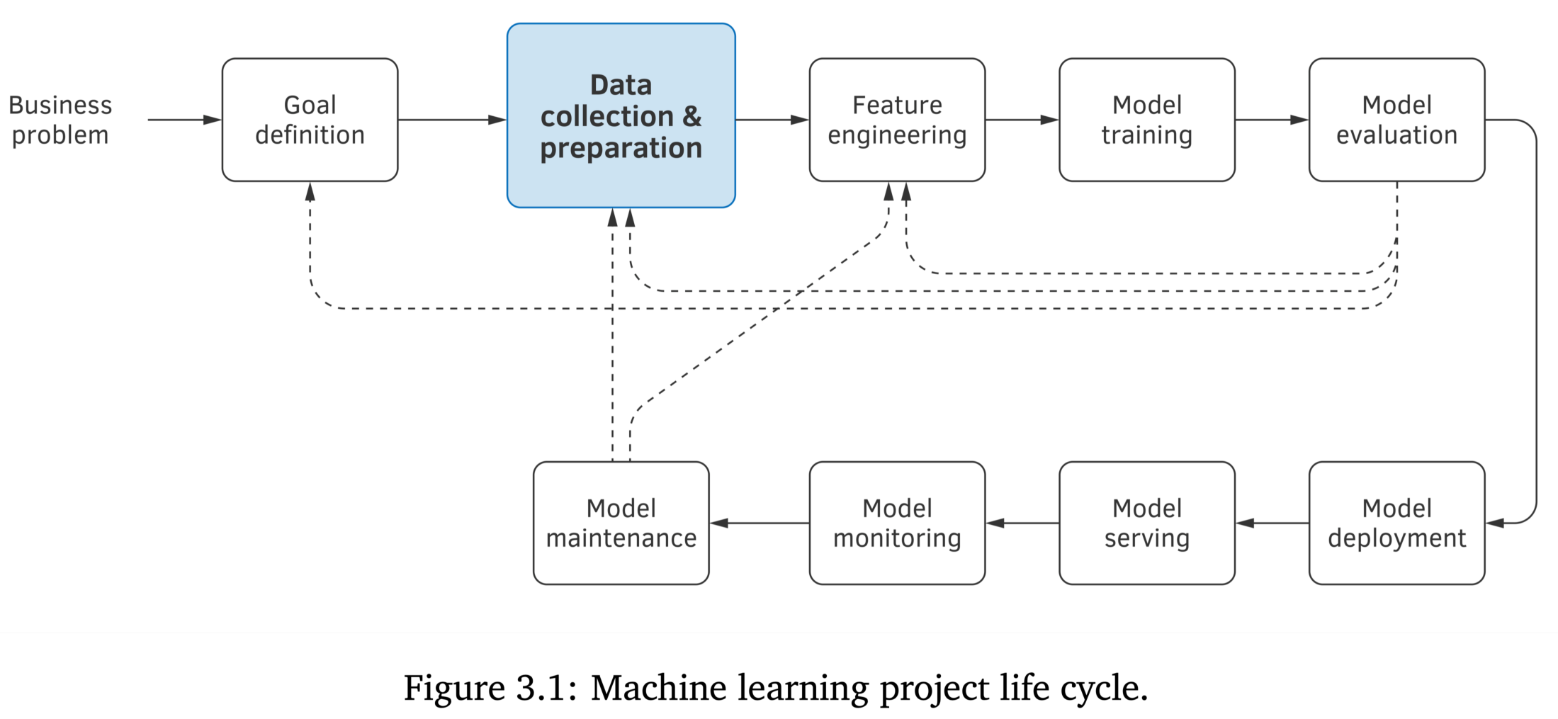
Machine Learning Engineering

Machine Learning Engineering

The courses SDS 3386: Data Science Lab and CSI 4142: Fundamentals of Data Science provide comprehensive coverage of machine learning engineering. This lecture introduces a focused subset of the preprocessing and feature-engineering concepts used in those courses.

As illustrated, the life cycle of a machine learning project typically involves multiple iterations. Each cycle enhances understanding of the problem and reveals limitations. Insufficient data quality often precipitates project failure.

Characteristics of High-Quality Data

• Volume: Is the dataset sufficiently large to support generalization?
• Relevance: Do the features accurately model the problem?
• Representation: Does the data reflect the conditions expected in production?
  • Are these features obtainable from real-world inputs?
  • Does the dataset adequately cover and represent feature examples?
• Bias: Is the data free from bias?
• Label Consistency: Are the labels consistent throughout the dataset?

Machine Learning Project Cycle

Gathering data and extracting features are the first two steps of a machine learning project.

1. Gather adequate data.
2. Extract features from the raw data:
   • This process is labor-intensive.
   • It necessitates creativity.
   • Domain knowledge is highly beneficial.

Attribution: Burkov (2020), Figure 3.1

Encoding

Why?

After completing Assignment 1, you generated a .csv file containing cleaned data.

Why would additional steps be necessary?

Dataset - Adult

import numpy as np
np.random.seed(42)

from sklearn.datasets import fetch_openml

adult = fetch_openml(name='adult', version=2)

print(adult.DESCR)

The ‘Adult’ dataset contains several attributes characterized by categorical values. This dataset will serve as a basis for a brief discussion on encoding these categorical values.

Dataset - Adult

Author: Ronny Kohavi and Barry Becker
Source: UCI - 1996
Please cite: Ron Kohavi, “Scaling Up the Accuracy of Naive-Bayes Classifiers: a Decision-Tree Hybrid”, Proceedings of the Second International Conference on Knowledge Discovery and Data Mining, 1996

Prediction task is to determine whether a person makes over 50K a year. Extraction was done by Barry Becker from the 1994 Census database. A set of reasonably clean records was extracted using the following conditions: ((AAGE>16) && (AGI>100) && (AFNLWGT>1)&& (HRSWK>0))

This is the original version from the UCI repository, with training and test sets merged.

Variable description

Variables are all self-explanatory except fnlwgt. This is a proxy for the demographic background of the people: “People with similar demographic characteristics should have similar weights”. This similarity-statement is not transferable across the 51 different states.

Description from the donor of the database:

The weights on the CPS files are controlled to independent estimates of the civilian noninstitutional population of the US. These are prepared monthly for us by Population Division here at the Census Bureau. We use 3 sets of controls. These are: 1. A single cell estimate of the population 16+ for each state. 2. Controls for Hispanic Origin by age and sex. 3. Controls by Race, age and sex.

We use all three sets of controls in our weighting program and “rake” through them 6 times so that by the end we come back to all the controls we used. The term estimate refers to population totals derived from CPS by creating “weighted tallies” of any specified socio-economic characteristics of the population. People with similar demographic characteristics should have similar weights. There is one important caveat to remember about this statement. That is that since the CPS sample is actually a collection of 51 state samples, each with its own probability of selection, the statement only applies within state.

Relevant papers

Ronny Kohavi and Barry Becker. Data Mining and Visualization, Silicon Graphics.
e-mail: ronnyk ‘@’ live.com for questions.

Downloaded from openml.org.

Adult - Workclass

adult.data['workclass'].unique()

['Private', 'Local-gov', NaN, 'Self-emp-not-inc', 'Federal-gov', 'State-gov', 'Self-emp-inc', 'Without-pay', 'Never-worked']
Categories (8, str): ['Federal-gov', 'Local-gov', 'Never-worked', 'Private', 'Self-emp-inc', 'Self-emp-not-inc', 'State-gov', 'Without-pay']

Adult - Education

adult.data['education'].unique()

['11th', 'HS-grad', 'Assoc-acdm', 'Some-college', '10th', ..., 'Assoc-voc', '9th', '12th', '1st-4th', 'Preschool']
Length: 16
Categories (16, str): ['10th', '11th', '12th', '1st-4th', ..., 'Masters', 'Preschool', 'Prof-school', 'Some-college']

Adult - Marital Status

adult.data['marital-status'].unique()

['Never-married', 'Married-civ-spouse', 'Widowed', 'Divorced', 'Separated', 'Married-spouse-absent', 'Married-AF-spouse']
Categories (7, str): ['Divorced', 'Married-AF-spouse', 'Married-civ-spouse', 'Married-spouse-absent', 'Never-married', 'Separated', 'Widowed']

Categorical Data

Key Points on Data Representation

• Numerical Representation: Many learning algorithms require numerical feature vectors.

• Meaning Matters: The representation should preserve whether categories are unordered or have an inherent order.

Encoding Methods

Consider the workclass attribute, which has 8 distinct values like ‘Federal-gov’, ‘Local-gov’, and so on.

• Which encoding method is preferable and why?

1. w = 1, 2, 3, 4, 5, 6, 7, or 8
2. w = [0,0,0], [0,0,1], [0,1,0], \ldots, or [1,1,1]
3. w = [1,0,0,0,0,0,0,0], [0,1,0,0,0,0,0,0], \ldots, or [0,0,0,0,0,0,0,1]

Encoding Nominal Data

One-hot encoding is a common default for unordered, or nominal, categories.

• Increases Dimensionality: One-hot encoding creates one output feature per retained category.
• Avoids Artificial Order: Integer codes can introduce distances and order that the categories do not possess.
• Example of Bias: Using the first method, w = 1, 2, 3, etc., implies that ‘Federal-gov’ and ‘Local-gov’ are similar, while ‘Federal-gov’ and ‘Without-pay’ are not.
• Misleading Similarity: The second method, w = [0,0,0], [0,0,1], etc., might mislead the algorithm by suggesting similarity based on numeric patterns.

Definition

One-Hot Encoding: A technique that converts categorical variables into a binary vector representation, where each category is represented by a vector with a single ‘1’ and all other elements as ‘0’.

High-cardinality attributes may require other representations, such as grouping infrequent categories, hashing, target encoding, or learned embeddings.

OneHotEncoder

from sklearn.preprocessing import OneHotEncoder

work = adult.data[['workclass']]

onehot_encoder = OneHotEncoder(handle_unknown="ignore")

onehot_encoder.fit(work)
values_encoded = onehot_encoder.transform(work)

values_encoded[:5].toarray()

array([[0., 0., 0., 1., 0., 0., 0., 0., 0.],
       [0., 0., 0., 1., 0., 0., 0., 0., 0.],
       [0., 1., 0., 0., 0., 0., 0., 0., 0.],
       [0., 0., 0., 1., 0., 0., 0., 0., 0.],
       [0., 0., 0., 0., 0., 0., 0., 0., 1.]])

An encoder learns the categories and their column order during fit. Fitting a second encoder on validation, test, or production data can therefore change the meaning or number of columns. The correct pattern is to fit the encoder on the training data and reuse its transform method everywhere else. A pipeline applies this pattern automatically during cross-validation.

While Pandas offers a method called get_dummies() for one-hot encoding, it is important to note the following distinctions:

• Category Memory: OneHotEncoder retains the categories it was trained on, whereas get_dummies() does not.
• Consistency in Production: It is crucial to use the same encoding scheme in production as was used during training to ensure accurate results.
• Vector Length Discrepancies: If get_dummies() encounters a different number of categories in new data, it will produce vectors of varying lengths, leading to potential errors.
• Handling Missing Values: By default, get_dummies() encodes a missing value as all zeros. An explicit missing-value column is created only with dummy_na=True.

Ensuring consistency in encoding across training, validation, and production datasets is essential to maintain the integrity and accuracy of your machine learning models.

Consistency is Key: Ensure you use the same encoding on: Validation Set, Test Set, and Production Data.

Case Study

• Dataset: Heart Disease
  • Examples: 303, features: 13
  • Target: 0 denotes absence; values 1–4 denote presence of disease
• Categorical Data:
  • sex: 1 = male, 0 = female
  • cp (chest pain type):
    • 1: Typical angina
    • 2: Atypical angina
    • 3: Non-anginal pain
    • 4: Asymptomatic
  • Other: ‘fbs’, ‘restecg’, ‘exang’, ‘slope’, ‘thal’

The UCI target records absence as 0 and degrees of presence as values 1 through 4. The code converts these values into the binary task described on the slide.

Dropped rows can differ systematically from complete rows, so this shortcut may introduce selection bias. A realistic analysis would investigate the missingness process and compare an imputation strategy fitted on the training data.

The example is intentionally limited to preprocessing. Model and regularization choices would be selected with validation data or cross-validation, while the test set would remain reserved for final evaluation.

To simplify the analysis: Examples with missing values are dropped, the target is converted to absence/presence, and no hyperparameter tuning is performed.

Case Study

import pandas as pd
import numpy as np
import matplotlib.pyplot as plt
from sklearn.datasets import fetch_openml
from sklearn.preprocessing import OneHotEncoder, StandardScaler
from sklearn.compose import ColumnTransformer
from sklearn.linear_model import LogisticRegression
from sklearn.model_selection import train_test_split
from sklearn.metrics import classification_report
from sklearn.pipeline import Pipeline

# Load the 'Heart-Disease' dataset from OpenML
data = fetch_openml(name='Heart-Disease', version=1, as_frame=True)
df = data.frame

# Replace '?' with NaN and convert columns to numeric
for col in df.columns:
    df[col] = pd.to_numeric(df[col], errors='coerce')

# Drop rows with missing values
df.dropna(inplace=True)

# Define features and convert the target to absence/presence
X = df.drop(columns=['target'])
y = (df['target'] > 0).astype(int)

# Columns to encode with OneHotEncoder
columns_to_encode = ['sex', 'cp', 'fbs', 'restecg', 'exang', 'slope', 'thal']

# Identify numerical columns
numerical_columns = X.columns.difference(columns_to_encode)

# Split the dataset into training and testing sets before transformations
X_train, X_test, y_train, y_test = train_test_split(
    X, y, test_size=0.2, random_state=42, stratify=y
)

# Apply OneHotEncoder and StandardScaler using ColumnTransformer
preprocessor = ColumnTransformer(
    transformers=[
        (
            'onehot',
            OneHotEncoder(drop='first', handle_unknown='ignore'),
            columns_to_encode,
        ),
        ('scaler', StandardScaler(), numerical_columns)
    ]
)

# The pipeline fits preprocessing and the classifier on training data only
heart_pipeline = Pipeline([
    ('preprocessor', preprocessor),
    ('classifier', LogisticRegression()),
])
heart_pipeline.fit(X_train, y_train)

ColumnTransformer applies different transformations to selected columns. Its transformer can also be drop, which excludes the selected columns, or passthrough, which retains them unchanged.

The surrounding Pipeline is the important engineering pattern: calling fit learns both the preprocessing parameters and the classifier from the training data. Calling predict applies the already-fitted transformations before classification. During cross-validation, each fold therefore learns its own preprocessing parameters from that fold’s training partition.

Case study - results

# Predict and evaluate on the untouched test set
y_pred = heart_pipeline.predict(X_test)

print(classification_report(y_test, y_pred))

              precision    recall  f1-score   support

           0       0.83      0.71      0.77        28
           1       0.78      0.88      0.83        33

    accuracy                           0.80        61
   macro avg       0.81      0.80      0.80        61
weighted avg       0.81      0.80      0.80        61

Case study - chest pain (cp)

# Retrieve feature names and coefficients from the fitted pipeline
feature_names = heart_pipeline[
    'preprocessor'
].get_feature_names_out()

coefficients = heart_pipeline['classifier'].coef_[0]

# Create a DataFrame with feature names and coefficients
coef_df = pd.DataFrame({
    'Feature': feature_names,
    'Coefficient': coefficients
})

# Display coefficients associated with 'cp'
cp_features = coef_df[coef_df['Feature'].str.contains('_cp')]
print("\nCoefficients associated with 'cp':")
print(cp_features)

Coefficients associated with 'cp':
          Feature  Coefficient
1  onehot__cp_1.0     0.754906
2  onehot__cp_2.0     1.440017
3  onehot__cp_3.0     1.255102

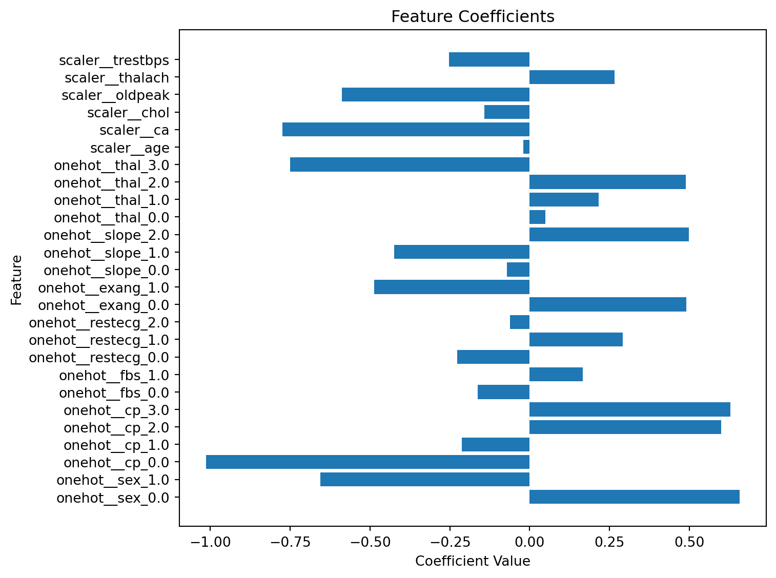
Case study - coefficients

# Visualize the fitted coefficients

coef_plot_df = coef_df.sort_values(by='Coefficient')
plt.figure(figsize=(8, 6))
plt.barh(coef_plot_df['Feature'], coef_plot_df['Coefficient'])
plt.title('Feature Coefficients')
plt.xlabel('Coefficient Value')
plt.ylabel('Feature')
plt.tight_layout()
plt.show()

With the first category of each encoded attribute used as a reference, a positive coefficient raises the fitted log-odds of heart-disease presence relative to that reference, holding the other transformed features fixed. A negative coefficient lowers those log-odds.

Coefficient magnitude also depends on feature scaling and regularization. These coefficients describe associations in this fitted model; they do not establish that a feature causes heart disease.

Definition

Ordinal encoding is a technique that assigns numerical values to categorical attributes based on their inherent order or rank.

Feature Engineering - Ordinal

For attributes with values such as ‘Poor’, ‘Average’, and ‘Good’, an ordinal encoding can preserve their ordering.

However!

from sklearn.preprocessing import OrdinalEncoder

X =[['Poor'], ['Average'], ['Good'], ['Average'], ['Average']]

encoder = OrdinalEncoder()

encoder.fit(X)
encoder.transform(X)

array([[2.],
       [0.],
       [1.],
       [0.],
       [0.]])

OrdinalEncoder (revised)

from sklearn.preprocessing import OrdinalEncoder

X =[['Poor'], ['Average'], ['Good'], ['Average'], ['Average']]

encoder = OrdinalEncoder(categories=[['Poor', 'Average', 'Good']])

encoder.fit(X)

X_encoded = encoder.transform(X)

X_encoded

array([[0.],
       [1.],
       [2.],
       [1.],
       [1.]])

The desired order of the categories must be explicitly provided to the encoder; otherwise, it defaults to alphabetical order.

An ordinal encoder is appropriate when categorical attributes have a clear, inherent order or ranking, such as ‘Low’, ‘Medium’, and ‘High’, or ‘Poor’, ‘Average’, and ‘Good’. This encoding method preserves the ordinal relationships among categories.

When data is inherently ordinal, this encoding is more compact and can be advantageous for machine learning models. However, if there is any uncertainty about the ordinal nature of the data, it is safer to use a OneHotEncoder.

Definition

Discretization maps a continuous or fine-grained numerical feature into a finite set of intervals.

AKA binning, bucketing, or quantization.

Feature Engineering: Binning

Example: Categorizing ages into bins such as ‘infant’, ‘child’, ‘teen’, ‘adult’, and ‘senior citizen’.

Possible advantage:

• Encodes useful domain thresholds and can reduce model complexity.

Disadvantages:

• Discards differences within each interval and introduces abrupt boundaries.
• Requires defensible cut points; for example, the starting age for ‘senior citizen’ could be 60, 65, or 70¹.

Predefined bins can help a decision tree produce a more compact model because the tree no longer has to discover every threshold from the available sample.

However, this strong inductive bias can hide useful variation or prevent the estimator from discovering better boundaries. Binning is therefore a modelling choice, not an automatic preprocessing step.

Cross-validation is an effective method to determine the best encoding scheme, but it is essential to withhold the test set until the final evaluation phase of the project to prevent data leakage and ensure unbiased assessment.

1. Your instructor is concerned with your choice of cutoff

FunctionTransformer

import pandas as pd
import numpy as np
from sklearn.preprocessing import FunctionTransformer

bins = [0, 1, 13, 20, 60, np.inf]
labels = ['infant', 'kid', 'teen', 'adult', 'senior citizen']

transformer = FunctionTransformer(
    pd.cut, kw_args={'bins': bins, 'labels': labels, 'retbins': False}
)

X = np.array([0.5, 2, 15, 25, 97])
transformer.fit_transform(X)

['infant', 'kid', 'teen', 'adult', 'senior citizen']
Categories (5, str): ['infant' < 'kid' < 'teen' < 'adult' < 'senior citizen']

See also: KBinsDiscretizer

Scaling

What is it?

Scaling attributes ensures that their values fall within comparable ranges.

Why?

Why do some estimators require comparable feature scales?

Scaling changes the geometry and numerical conditioning of a learning problem. Whether it helps depends on the estimator.

Distance-based methods such as k-nearest neighbours and k-means are sensitive because a large-scale feature can dominate the distance. RBF kernels and regularized linear models are also scale-sensitive. Gradient-based optimization often converges more readily when feature scales are comparable.

Tree-based models make threshold comparisons within one feature at a time, so monotonic rescaling usually leaves their possible partitions unchanged.

Scaling does not decide how important a feature should be. Domain knowledge and the model’s intended geometry still matter.

Scenario

We pretend to predict a house price using k-Nearest Neighbors (KNN) regression with two features:

• x_1: number of rooms (small scale)
• x_2: square footage (large scale)

Data (three houses)

import numpy as np
import pandas as pd

# Three examples (rooms, sqft); prices only for b and c (training)
point_names = ["a", "b", "c"]
X = np.array([
    [4, 1500.0],  # a (query)
    [8, 1520.0],  # b (train)
    [4, 1300.0],  # c (train)
], dtype=float)

prices = pd.Series([np.nan, 520_000, 390_000], index=point_names, name="price")

df = pd.DataFrame(X, columns=["rooms", "sqft"], index=point_names)
display(df)
display(prices.to_frame())

Note. We’ll treat b and c as the training set, and a as the query whose price we want to predict.

Data (three houses)

	rooms	sqft
a	4.0	1500.0
b	8.0	1520.0
c	4.0	1300.0

	price
a	NaN
b	520000.0
c	390000.0

Euclidean distances (unscaled)

When one feature has a much larger scale (e.g., square footage), it can dominate the sum.

from sklearn.metrics import pairwise_distances

dist_unscaled = pd.DataFrame(
    pairwise_distances(df.values, metric="euclidean"),
    index=df.index, columns=df.index
)
dist_unscaled

print("Nearest to 'a' (unscaled):", dist_unscaled.loc["a"].drop("a").idxmin())

Nearest to 'a' (unscaled): b

Euclidean distances (unscaled)

	a	b	c
a	0.000000	20.396078	200.000000
b	20.396078	0.000000	220.036361
c	200.000000	220.036361	0.000000

Proper scaling for modeling

For a fair ML workflow, compute scaling parameters on the training data (b, c) only, then transform both train and query:

from sklearn.preprocessing import StandardScaler

train_idx = ["b", "c"]
query_idx = ["a"]

scaler = StandardScaler()

scaler.fit(df.loc[train_idx])     # fit only on training points

Z = pd.DataFrame(
    scaler.transform(df),
    columns=df.columns, index=df.index
)

Z

Proper scaling for modeling

	rooms	sqft
a	-1.0	0.818182
b	1.0	1.000000
c	-1.0	-1.000000

Euclidean distances (after scaling)

dist_scaled = pd.DataFrame(
    pairwise_distances(Z.values, metric="euclidean"),
    index=Z.index, columns=Z.index
)
dist_scaled

	a	b	c
a	0.000000	2.008247	1.818182
b	2.008247	0.000000	2.828427
c	1.818182	2.828427	0.000000

print("Nearest to 'a' (scaled):", dist_scaled.loc["a"].drop("a").idxmin())

Nearest to 'a' (scaled): c

KNN regressor

A 1-NN regressor predicts the price of the nearest training example. Compare the same estimator with and without scaling.

from sklearn.neighbors import KNeighborsRegressor

X_train = df.loc[train_idx].values
y_train = prices.loc[train_idx].values
X_query = df.loc[query_idx].values

knn_plain = KNeighborsRegressor(n_neighbors=1, metric="euclidean")
knn_plain.fit(X_train, y_train)

knn_scaled = Pipeline([
    ("scaler", StandardScaler()),
    ("knn", KNeighborsRegressor(n_neighbors=1, metric="euclidean"))
])

knn_scaled.fit(X_train, y_train)

The pipeline behaves like a single regressor. Its fit method learns the scaler from X_train and then fits KNN in the transformed space. Its predict method applies that fitted scaler before searching for neighbours.

KNN regressor: results

pred_plain = knn_plain.predict(X_query)[0]
pred_scaled = knn_scaled.predict(X_query)[0]

plain_index = knn_plain.kneighbors(
    X_query, return_distance=False
)[0, 0]
scaled_query = knn_scaled["scaler"].transform(X_query)
scaled_index = knn_scaled["knn"].kneighbors(
    scaled_query, return_distance=False
)[0, 0]

knn_comparison = pd.DataFrame(
    {
        "prediction": [pred_plain, pred_scaled],
        "nearest neighbour": [
            train_idx[plain_index], train_idx[scaled_index]
        ],
    },
    index=["without scaling", "with scaling"],
)

	Prediction	Nearest neighbour
Without scaling	$520,000	b
With scaling	$390,000	c

This deliberately tiny dataset illustrates geometry, not model quality. Two observations are not enough to estimate stable population means and standard deviations, and the query has no known price with which to measure predictive performance. The example demonstrates a change in neighbour and prediction, not an improvement in accuracy.

Min-max scaling

Min-max scaling maps each feature to a chosen interval, usually [0,1].

\frac{x_i^{(j)} - \min^{(j)}}{\max^{(j)} - \min^{(j)}}

The minimum and maximum must be learned from the training data.

See: sklearn.preprocessing.MinMaxScaler

Standardization

Standardization subtracts the training mean and divides by the training standard deviation.

\frac{x_i^{(j)} - \mu^{(j)}}{\sigma^{(j)}}

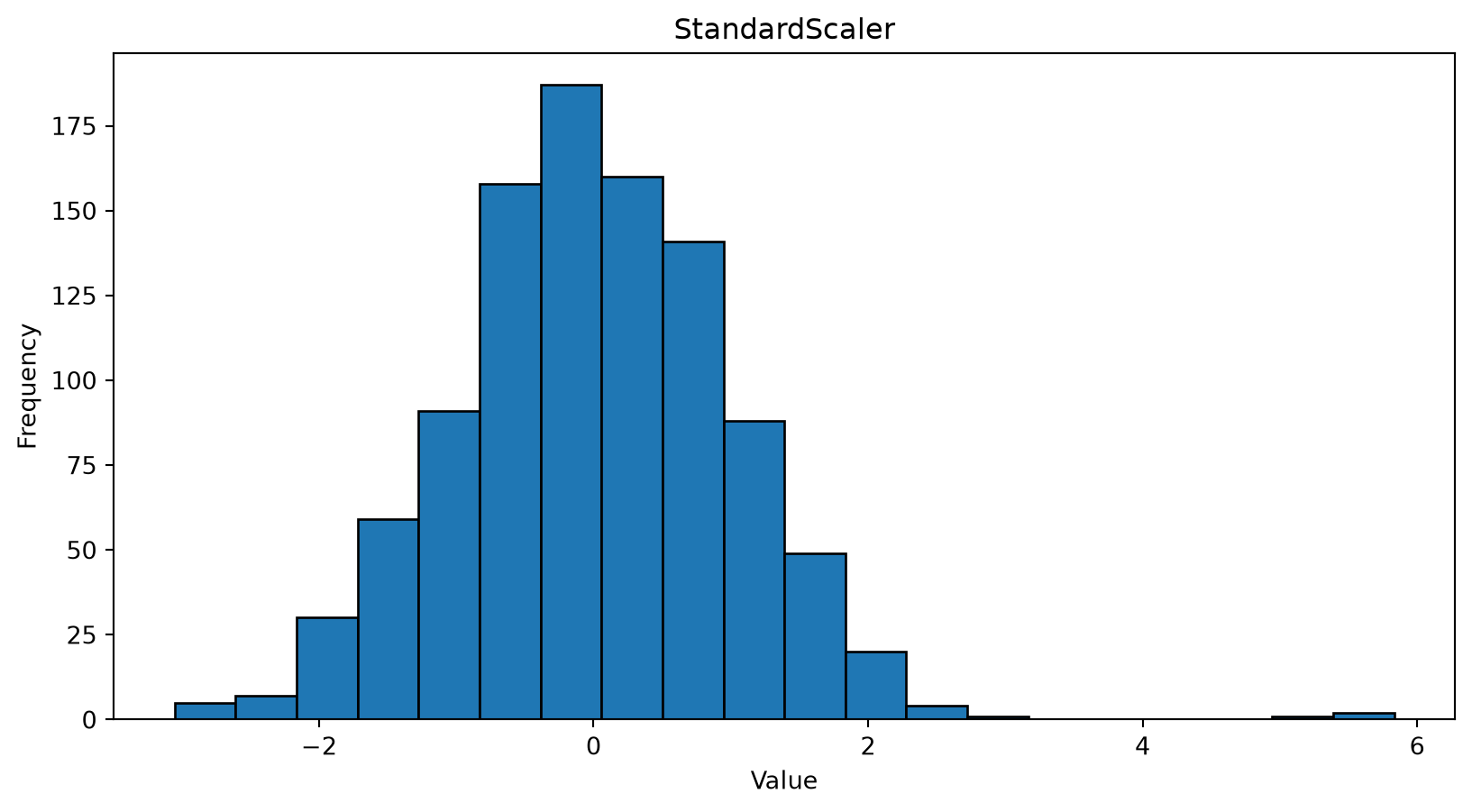
The transformed training feature has mean 0 and variance 1, but its distribution does not become normal and its range is not bounded.

See: sklearn.preprocessing.StandardScaler

Choosing a scaling method

• Standardization is a common choice for distance-based methods, regularized linear models, and gradient-based optimization.
• Min-max scaling is useful when a bounded input range is required.
• Both methods are sensitive to outliers: min-max scaling uses extremes, while standardization uses the mean and standard deviation.
• For strongly skewed features or outliers, investigate the data-generating process and consider a justified transformation, clipping rule, or RobustScaler.
• If several choices are plausible and consequential, compare them within cross-validation.

Scaling and distributional transformation solve different problems. A logarithm can reduce right skew for strictly positive data, but it must be meaningful for the feature and fitted into the same leakage-safe workflow. RobustScaler uses the median and interquartile range, which makes its fitted statistics less sensitive to extreme values.

Scaling methods compared

Feature	Standardization	Min-max scaling
Output Range	Not bounded	Typically [0, 1]
Center	Mean at 0	Not centered
Outlier sensitivity	Sensitive through the mean and standard deviation	Sensitive through the minimum and maximum
Typical use	Comparable variance and zero-centred features	A prescribed bounded range

Avoid Data Leakage!

The correct workflow:

• Split the examples before learning any preprocessing parameters.
• Fit the scaler on the training data.
• Reuse that fitted scaler to transform validation, test, and production data.
• During cross-validation, fit preprocessing separately inside each training fold—normally by placing it in a Pipeline.

Means, standard deviations, minima, maxima, category sets, and imputation values are all learned information. They must come from the training data only.

The test set simulates unseen data. Allowing it to influence preprocessing gives the training procedure information that would not be available when making a genuinely new prediction. This data leakage can produce an optimistic estimate of generalization performance.

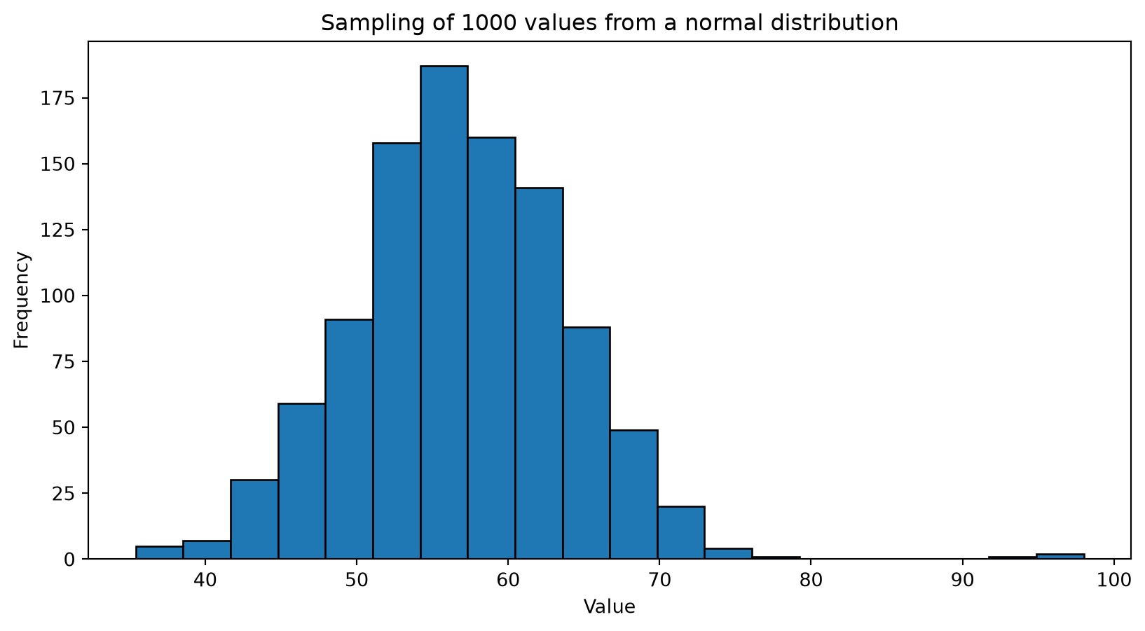
Normally distributed sample with outliers

import numpy as np
np.random.seed(7)

# Sample characteristics
sample_size = 1000
mu = 57
sigma = 7

# Generate values
norm_values = sigma * np.random.randn(sample_size) + mu

# Add three outliers
norm_values = np.append(norm_values, [92, 95, 98])

Original distribution

import matplotlib.pyplot as plt

# Plot the histogram
plt.hist(norm_values, bins=20, edgecolor='black')

plt.title(f'Sampling of {sample_size} values from a normal distribution')

plt.xlabel('Value')
plt.ylabel('Frequency')

plt.show()

Min-max scaling

from sklearn.preprocessing import MinMaxScaler

scaler = MinMaxScaler()

minmax_norm_values = scaler.fit_transform(norm_values.reshape(-1, 1))

# Plot the histogram
plt.hist(minmax_norm_values, bins=20, edgecolor='black')

plt.title(f'MinMaxScaler')

plt.xlabel('Value')
plt.ylabel('Frequency')

plt.show()

The largest observed value is mapped to 1 and the smallest to 0. The high outliers stretch that interval, compressing most observations into its lower portion. Min-max scaling does not imply that the transformed mean should be 0.5.

Min-max scaling of values from a normal distribution containing high outliers.

Standardization

standard_scaler = StandardScaler()

standard_norm_values = standard_scaler.fit_transform(
    norm_values.reshape(-1, 1)
)

# Plot the histogram
plt.hist(standard_norm_values, bins=20, edgecolor='black')

plt.title(f'StandardScaler')

plt.xlabel('Value')
plt.ylabel('Frequency')

plt.show()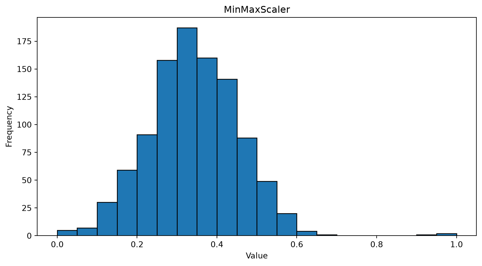

Standardization changes the centre and scale but preserves the distribution’s shape. The bulk of this approximately normal sample lies near zero, while the outliers remain outliers. The interval [-2,2] is a useful empirical description for this sample, not a guarantee of StandardScaler.

Standardization (StandardScaler) of values from a normal distribution containing outliers.

Missing Values

Definition

Missing values refer to the absence of data points or entries in a dataset where a value is expected.

Age is a good example, as some patients may withhold their age due to privacy concerns.

Handling Missing Values

• Drop Examples
  • Reasonable only when enough data remain and the missing rows are not systematically different.
• Drop Features
  • Suitable when a feature is not essential and too little reliable information remains.
• Use Algorithms Handling Missing Data
  • Some estimators model missing values directly; many others do not accept them.
• Data Imputation
  • Replace missing values using statistics or a model learned from the training data.

Definition

Data imputation is the process of replacing missing values in a dataset with substituted values, typically using statistical or machine learning methods.

Data Imputation Strategy

Replace missing numerical values with the training mean or median of the feature.

from sklearn.impute import SimpleImputer

X_train_missing = np.array([
    [1.0, 10.0],
    [2.0, np.nan],
    [3.0, 12.0],
])
X_new_missing = np.array([[4.0, np.nan]])

imputer = SimpleImputer(strategy="median")
imputer.fit(X_train_missing)
imputer.transform(X_new_missing)

array([[ 4., 11.]])

• Limitation: Univariate imputation ignores relationships between features and reduces the observed variability.

• Categorical Features: Use the most frequent category or an explicit "missing" category when that representation is appropriate.

Missingness can be completely at random, related to other observed features, or related to the missing value itself. These mechanisms are often described as MCAR, MAR, and MNAR. A simple imputer does not determine which mechanism produced the missing values.

Mean, median, and most-frequent imputation are useful baselines, but they can distort distributions and relationships. The imputation strategy is part of the model and must be assessed on held-out data.

As with scaling, fit the imputer only on the training partition. A pipeline repeats that fit correctly within every cross-validation fold.

Preserve Missingness Information

An imputed value can be accompanied by a binary feature indicating that the original value was missing.

imputer_with_indicator = SimpleImputer(
    strategy="median", add_indicator=True
)
imputer_with_indicator.fit_transform(X_train_missing)

array([[ 1., 10.,  0.],
       [ 2., 11.,  1.],
       [ 3., 12.,  0.]])

add_indicator=True lets an estimator use the fact that a value was missing as a separate signal. This can help when the observation process is informative—for example, when one measurement is ordered only for higher-risk patients.

A sentinel value outside the normal range can serve a similar purpose for some tree-based models, but it can badly distort distances or linear relationships. An explicit indicator communicates the intent more clearly.

Predict a Missing Feature

• Select a feature containing missing values as the prediction target.
• Use rows where that feature is observed as training examples.
• Use the remaining observed features as inputs.
• Predict the missing entries with a regression or classification model.

Using ML for Imputation

1. Neighbour-Based Method:

   • Use k nearest neighbors (k-NN) to find the k closest examples and impute using the non-missing values from the neighborhood.

2. Iterative Model-Based Methods:

   • Predict each incomplete feature from the others and repeat the process across features.

Consult the scikit-learn imputation guide or KNNImputer documentation.

Why Use these Methods?

• Possible advantage:
  • Can use relationships between features that univariate imputation ignores.
• Limitations:
  • More computation and modelling choices do not guarantee better predictions.
  • The imputer must still be fitted inside each training split or cross-validation fold.

Class Imbalance Remedies

From Evaluation to Intervention

Lecture 7 established that class imbalance can hide poor performance on an infrequent class and that evaluation must reflect the decision problem.

This lecture asks a different question:

How can the training procedure respond to class imbalance without contaminating evaluation?

Lecture 7 already developed the confusion matrix, accuracy, precision, recall, F_1, micro and macro averaging, threshold trade-offs, ROC curves, and precision–recall curves. Those definitions and formulas are not repeated here.

The important transition is from detecting a problem during evaluation to changing the training procedure. A remedy is useful only if it improves the application-relevant validation measure established in Lecture 7.

Training-Time Remedies

• Class or sample weights: Make errors on selected examples contribute more strongly to the training objective.
• Random oversampling: Repeat minority-class training examples.
• Random undersampling: Retain fewer majority-class training examples.
• SMOTE: Interpolate synthetic minority-class examples from neighbouring training examples.
• Decision threshold: Select an operating point using validation data, as introduced in Lecture 7.

Class weights change the contribution of training examples without creating or deleting observations. Oversampling can overfit repeated examples, whereas undersampling can discard useful majority-class variation.

SMOTE constructs synthetic points between minority-class neighbours (Chawla et al. 2002). This interpolation can be inappropriate when a straight line between two observations leaves the set of plausible examples. Ordinary SMOTE also assumes numerical features; mixed numerical and categorical data require an appropriate variant such as SMOTENC.

No remedy is universally best. Compare plausible choices using the validation procedure and application-relevant measures established in Lecture 7.

Implementations: class_weight and imbalanced-learn.

Keep Evaluation Untouched

• Preserve the natural class distribution in validation and test data.
• Apply resampling only to a training partition.
• During cross-validation, resample separately inside each training fold.
• Place resampling and the estimator in an imbalanced-learn pipeline.
• Reserve the test set for the final evaluation after selecting the remedy and any decision threshold.

Resampling before the train/test split leaks information and also creates an unrealistic evaluation distribution. Resampling once before cross-validation has the same problem because a synthetic or repeated example can influence both training and validation folds.

An imbalanced-learn pipeline calls the sampler only while fitting each training fold. Its prediction path does not resample validation, test, or production examples.

New Features

Definition

Feature engineering is the process of creating, transforming, and selecting variables (attributes) from raw data to improve the performance of machine learning models.

Here, our focus is on creating new attributes from raw data.

Exploration

import numpy as np

np.random.seed(42)

X = 6 * np.random.rand(100, 1) - 3
y = 0.5 * X ** 2 - X + 2 + np.random.randn(100, 1)

import matplotlib as mpl
import matplotlib.pyplot as plt

plt.figure(figsize=(6,4))

plt.plot(X, y, "b.")
plt.xlabel("$x$", fontsize=18)
plt.ylabel("$y$", rotation=0, fontsize=18)
plt.axis([-3, 3, 0, 10])
plt.grid(True)
plt.show()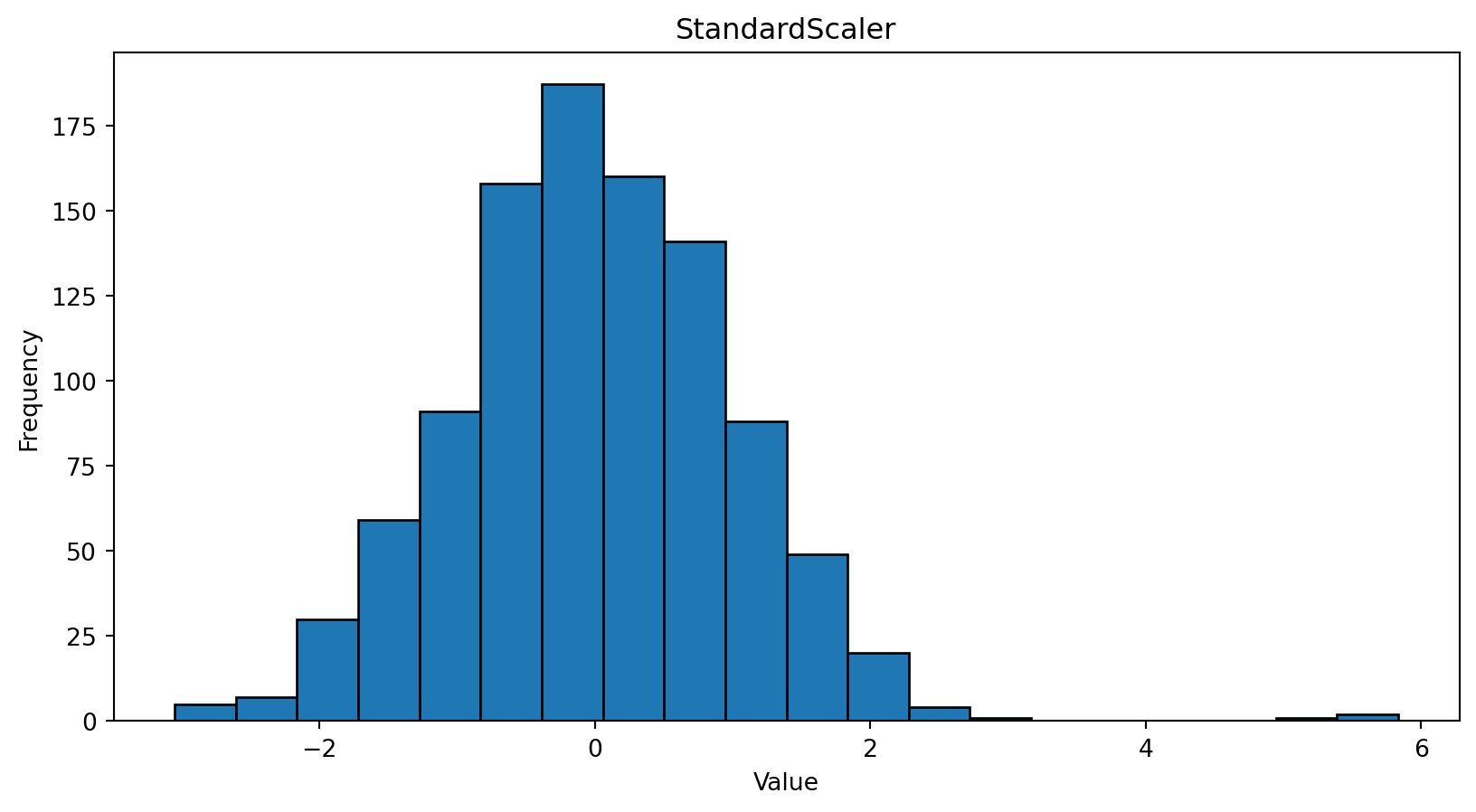

The scatter plot has a curved trend: the response decreases and then increases as x changes. A model that uses only an intercept and the original feature x cannot represent that curvature.

The fixed random seed makes the generated sample reproducible. Reproducibility is useful for comparing models and debugging, but a single seed does not establish that a result is stable across possible samples.

Attribution: Géron (2022), Chapter 4

Linear Regression

from sklearn.linear_model import LinearRegression

lin_reg = LinearRegression()
lin_reg.fit(X, y)

X_new = np.array([[-3], [3]])
y_pred = lin_reg.predict(X_new)

plt.figure(figsize=(6,4))

plt.plot(X, y, "b.")
plt.plot(X_new, y_pred, "r-")
plt.xlabel("$x$", fontsize=18)
plt.ylabel("$y$", rotation=0, fontsize=18)
plt.axis([-3, 3, 0, 10])
plt.show()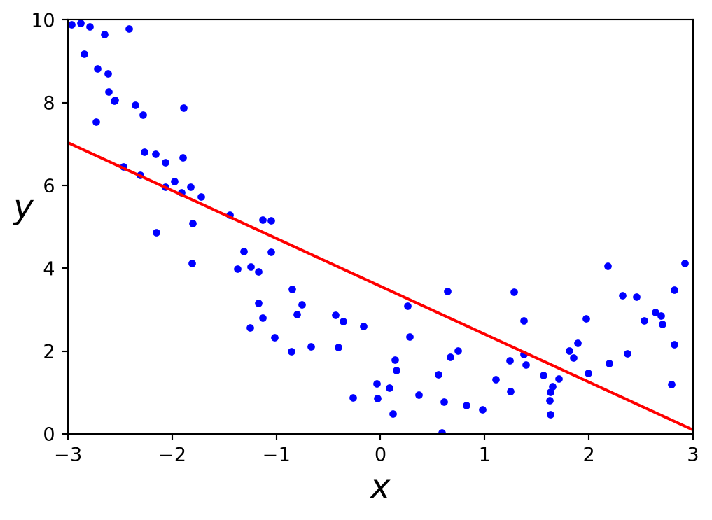

A linear model inadequately represents this dataset.

The best-fitting straight line balances residuals across the dataset, but changing its slope and intercept cannot create a turning point. The model is underfitting because its representation is too restrictive for the observed relationship.

PolynomialFeatures

from sklearn.preprocessing import PolynomialFeatures

poly_features = PolynomialFeatures(degree=2, include_bias=False)
X_poly = poly_features.fit_transform(X)

X[0]

array([-0.75275929])

X_poly[0]

array([-0.75275929,  0.56664654])

sklearn.preprocessing.PolynomialFeatures

Generate a new feature matrix consisting of all polynomial combinations of the features with degree less than or equal to the specified degree. For example, if an input sample is two dimensional and of the form [a, b], the degree-2 polynomial features are [1, a, b, a^2, ab, b^2].

PolynomialFeatures

Given two features a and b, PolynomialFeatures with degree=3 would add a^2, a^3, b^2, b^3, as well as, ab, a^2b, ab^2!

Warning

With include_bias=True, the total number of output features is

\binom{D+d}{d} = \frac{(D+d)!}{d!D!},

where D is the number of input features. With include_bias=False, subtract one.

The output count includes the original features as well as powers and interactions. It grows quickly with both D and d, which increases computation and the risk of overfitting. Select the degree with validation and use regularization when appropriate.

Polynomial Regression

lin_reg = LinearRegression()
lin_reg = lin_reg.fit(X_poly, y)

X_new = np.linspace(-3, 3, 100).reshape(100, 1)
X_new_poly = poly_features.transform(X_new)
y_new = lin_reg.predict(X_new_poly)

plt.figure(figsize=(5, 3))
plt.plot(X, y, "b.")
plt.plot(X_new, y_new, "r-", linewidth=2, label="Predictions")
plt.xlabel("$x_1$")
plt.ylabel("$y$", rotation=0)
plt.legend(loc="upper left")
plt.axis([-3, 3, 0, 10])
plt.grid()
plt.show()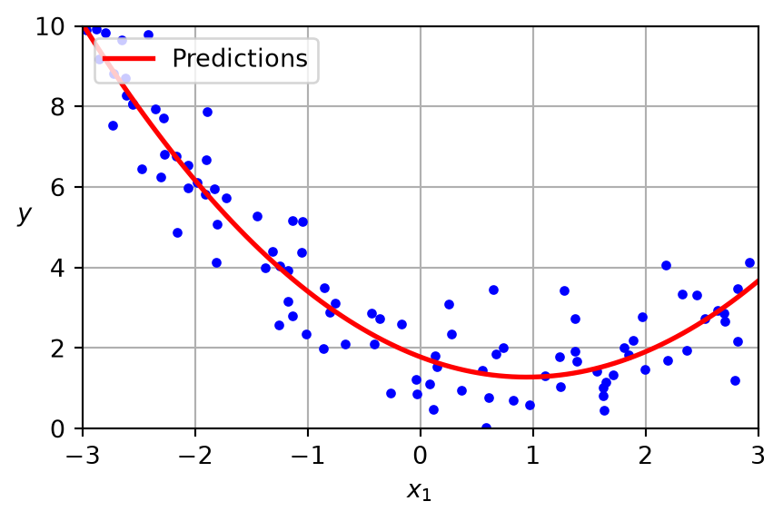

LinearRegression fitted to features [x, x^2].

Learned Polynomial

The data was generated according to the following equation, with the inclusion of Gaussian noise.

y = 0.5 x^2 - 1.0 x + 2.0

Presented below is the learned model.

\hat{y} = 0.56 x^2 + (-1.06) x + 1.78

lin_reg.coef_, lin_reg.intercept_

(array([[-1.06633107,  0.56456263]]), array([1.78134581]))

Linearity refers to the fitted coefficients, not necessarily to the original input. After defining z_1=x and z_2=x^2, linear regression fits

\hat{y}=\theta_0+\theta_1z_1+\theta_2z_2.

This expression is linear in \theta_0,\theta_1,\theta_2, even though it traces a curve as x changes. PolynomialFeatures changes the feature representation; it does not change the fitting algorithm into a different kind of regression estimator.

The fitted coefficients are close to the generating coefficients because the model contains the relevant quadratic term and the sample contains moderate Gaussian noise. Exact recovery is neither expected nor required.

Data Quantity and Augmentation

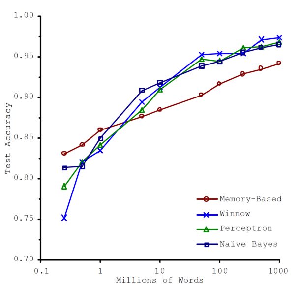
Size does matter

For the language task studied by Banko and Brill, increasing the training corpus produced large gains across several learning algorithms.

The result in Banko and Brill (2001) concerns one natural-language disambiguation task and should not be read as a universal law that more examples always solve a learning problem.

Additional data help when they provide relevant, correctly labelled, and representative information. More examples do not repair a mismatched target, systematic label errors, omitted subpopulations, or a distribution shift between training and deployment.

For some large neural models, empirical scaling laws relate loss to training data, parameter count, and computation over a studied range (Kaplan et al. 2020). Those regularities do not remove the need to examine data quality and coverage.

Attribution: Banko and Brill (2001)

Definition

Data augmentation creates additional training examples with transformations that should preserve the target label.

Purpose: Encode plausible invariances and improve robustness to variation expected in deployment.

Data Augmentation

• Images: Rotations, translations, crops, flips, or noise—when these transformations preserve the label.
  • How to find ancient geoglyphs using machine learning?, Sakai et al. (2024)
• Text: Carefully controlled paraphrasing or edits that preserve meaning and the assigned label.

An augmentation is valid only when its transformation preserves the target for the application. A horizontal flip may be harmless for many object categories but invalid for text, medical laterality, or traffic signs. Synonym replacement can also change nuance or grammar.

Apply augmentation only to training examples and, during cross-validation, only within the training fold. Validation and test sets should represent naturally occurring inputs.

Synthetic data require the same scrutiny as collected data. Indiscriminate reuse of model-generated content can narrow the represented distribution or amplify artifacts; Shumailov et al. (2024) discusses one form of this risk.

Generative models can also produce synthetic examples, but realistic-looking output does not guarantee correct labels, representative coverage, or independence from the source data.

Conclusion

Further readings

• Machine Learning Engineering by Andriy Burkov (Burkov 2020).
• Covers data collection, storage, preprocessing, feature engineering, model testing and debugging, deployment, retirement, and maintenance.
• From the author of The Hundred-Page Machine Learning Book (Burkov 2019).
• Available under a “read first, buy later” model.

Summary

• Match categorical encodings to nominal or ordinal meaning.
• Fit scaling, encoding, and imputation on training data through a pipeline.
• Choose scaling according to the estimator; scaling does not make a feature normally distributed.
• Apply class-imbalance remedies only within training partitions and evaluate on the natural distribution.
• Use polynomial and interaction features to expand a model’s representation while controlling complexity.
• Value representative, correctly labelled data and use only label-preserving augmentation.

Next lecture

• Next: artificial neural networks.

References

Banko, Michele, and Eric Brill. 2001. “Scaling to Very Very Large Corpora for Natural Language Disambiguation.” Proceedings of the 39th Annual Meeting on Association for Computational Linguistics (USA), ACL ’01, 26–33. https://doi.org/10.3115/1073012.1073017.

Burkov, A. 2020. Machine Learning Engineering. True Positive Incorporated. https://books.google.ca/books?id=HeXizQEACAAJ.

Burkov, Andriy. 2019. The Hundred-Page Machine Learning Book. Andriy Burkov.

Chawla, N V, K W Bowyer, L O Hall, and W P Kegelmeyer. 2002. “SMOTE: Synthetic minority over-sampling technique.” Journal of Artificial Intelligence Research 16: 321–57.

Géron, Aurélien. 2022. Hands-on Machine Learning with Scikit-Learn, Keras, and TensorFlow. 3rd ed. O’Reilly Media, Inc.

Halevy, Alon, Peter Norvig, and Fernando Pereira. 2009. “The Unreasonable Effectiveness of Data.” IEEE Intelligent Systems 24 (2): 8–12.

Kaplan, Jared, Sam McCandlish, Tom Henighan, et al. 2020. Scaling Laws for Neural Language Models. https://arxiv.org/abs/2001.08361.

Sakai, Masato, Akihisa Sakurai, Siyuan Lu, et al. 2024. “AI-accelerated Nazca survey nearly doubles the number of known figurative geoglyphs and sheds light on their purpose.” Proceedings of the National Academy of Sciences 121 (40): e2407652121. https://doi.org/10.1073/pnas.2407652121.

Shumailov, Ilia, Zakhar Shumaylov, Yiren Zhao, Nicolas Papernot, Ross Anderson, and Yarin Gal. 2024. “AI models collapse when trained on recursively generated data.” Nature 631 (8022): 755–59. https://doi.org/10.1038/s41586-024-07566-y.

Appendix: Video

Unreasonable Effectiveness of Data

Peter Norvig’s presentation runs for just over one hour and is provided for independent study rather than classroom viewing. The associated 2009 paper predates the modern wave of large deep-learning systems but remains useful for examining the relationship between data scale and modelling choices.

Supplementary presentation related to Halevy et al. (2009) and later empirical scaling work such as Kaplan et al. (2020).

Appendix: Pipeline

Pipeline

from sklearn.compose import ColumnTransformer, make_column_selector
from sklearn.impute import SimpleImputer
from sklearn.linear_model import LogisticRegression
from sklearn.pipeline import Pipeline
from sklearn.preprocessing import OneHotEncoder, StandardScaler

numeric_pipeline = Pipeline([
    ('imputer', SimpleImputer(strategy="median", add_indicator=True)),
    ('scaler', StandardScaler()),
])

preprocessor = ColumnTransformer([
    (
        "numeric",
        numeric_pipeline,
        make_column_selector(dtype_include=np.number),
    ),
    (
        "categorical",
        OneHotEncoder(handle_unknown="ignore"),
        make_column_selector(dtype_exclude=np.number),
    ),
])

full_pipeline = Pipeline([
    ("preprocessor", preprocessor),
    ("classifier", LogisticRegression()),
])

This template keeps every learned preprocessing step with the estimator. Numerical columns are imputed and standardized; categorical columns are one-hot encoded. The selectors choose columns by data type, so the template does not depend on lecture-specific column names.

Calling full_pipeline.fit(X_train, y_train) fits every component on the same training examples. The fitted pipeline can then transform and classify validation, test, or production examples consistently.

Marcel Turcotte

[email protected]

School of Electrical Engineering and Computer Science (EECS)

University of Ottawa