Introduction to Artificial Neural Networks

CSI 4106 - Fall 2025

Marcel Turcotte

Version: Oct 8, 2025 13:16

Preamble

Message of the Day

Message of the Day (2024)

Learning objectives

Explain perceptrons and MLPs: structure, function, history, and limitations.
Describe activation functions: their role in enabling complex pattern learning.
Implement a feedforward neural network with Keras on Fashion-MNIST.
Interpret neural network training and results: visualization and evaluation metrics.
Familiarize with deep learning frameworks: PyTorch, TensorFlow, and Keras for model building and deployment.

Introduction

TensorFlow Playground

Neural Networks (NN)

We now shift our focus to a family of machine learning models that draw inspiration from the structure and function of biological neural networks found in animals.

Machine Learning Problems

Supervised Learning: Classification, Regression
Unsupervised Learning: Autoencoders, Self-Supervised
Reinforcement Learning: Now an Integral Component

A neuron

Interconnected neurons

Connectionist

Hierarchy of concepts

Basics

Computations with neurodes

where \(x_1, x_2 \in \{0,1\}\) and \(f(z)\) is an indicator function: \[ f(z)= \begin{cases}0, & z<\theta \\ 1, & z \geq \theta\end{cases} \]

To better understand the development of modern neural networks, it is instructive to examine two earlier implementations that laid the groundwork for current advancements. This brief retrospective aims to introduce fundamental concepts relevant to contemporary networks. In this analysis, we will primarily focus on the computational aspects of neural networks, reserving the discussion on learning mechanisms for further exploration.

In mathematics, \(f(z)\), as defined above, is known as an indicator function or a characteristic function.

These neurodes have one or more binary inputs, taking a value of 0 or 1, and one binary output.

They showed that such units could implement Boolean functions such as AND, OR, and NOT.

But also that networks of such units can compute any logical proposition.

Computations with neurodes

\[ y = f(x_1 + x_2)= \begin{cases}0, & x_1 + x_2 <\theta \\ 1, & x_1 + x_2 \geq \theta\end{cases} \]

With \(\theta = 2\), the neurode implements an AND logic gate.
With \(\theta = 1\), the neurode implements an OR logic gate.

Computations with neurodes

Digital computations can be broken down into a sequence of logical operations, enabling neurode networks to execute any computation.
McCulloch and Pitts (1943) did not focus on learning parameter \(\theta\).
They introduced a machine that computes any function but cannot learn.

Perceptron

Threshold logic unit

In 1957, Frank Rosenblatt developed a conceptually distinct model of a neuron known as the threshold logic unit, which he published in 1958.

In this model, both the inputs and the output of the neuron are represented as real values. Notably, each input connection has an associated weight.

The left section of the neuron, denoted by the sigma symbol, represents the computation of a weighted sum of its inputs, expressed as \(\theta_1 x^{(1)} + \theta_2 x^{(2)} + \ldots + \theta_D x^{(D)} + b\).

This sum is then processed through a step function, right section of the neuron, to generate the output.

Here, \(x^T \theta\) represents the dot product of two vectors: \(x\) and \(\theta\). Here, \(x^T\) denotes the transpose of the vector \(x\), converting it from a row vector to a column vector, allowing the dot product operation to be performed with the vector \(\theta\).

The dot product \(x^T \theta\) is then a scalar given by:

\[ x^T \theta = x^{(1)} \theta_1 + x^{(2)} \theta_2 + \cdots + x^{(D)} \theta_D \]

where \(x^{(j)}\) and \(theta_j\) are the components of the vectors \(x\) and \(\theta\), respectively.

Simple Step Functions

\(\text{heaviside}(t)\) =

1, if \(t \geq 0\)
0, if \(t < 0\)

\(\text{sign}(t)\) =

1, if \(t > 0\)
0, if \(t = 0\)
-1, if \(t < 0\)

Notation

Notation

Perceptron

Perceptron

Classification tasks, can be further divided into multilabel and multiclass classification.

Multiclass Classification:
- In multiclass classification, each instance is assigned to one and only one class out of a set of three or more possible classes. The classes are mutually exclusive, meaning that an instance cannot belong to more than one class at the same time.
- Example: Classifying an image as either a cat, dog, or bird. Each image can only belong to one of these categories.
Multilabel Classification:
- In multilabel classification, each instance can be associated with multiple classes simultaneously. The classes are not mutually exclusive, allowing for the possibility that an instance can belong to several classes at once.
- Example: Tagging an image with multiple attributes such as “outdoor,” “sunset,” and “beach.” The image can simultaneously belong to all these labels.

The key difference lies in the relationship between classes: multiclass classification deals with a single label per instance, while multilabel classification handles multiple labels for each instance.

Notation

Notation

\(X\) is the input data matrix where each row corresponds to an example and each column represents one of the \(D\) features.
\(W\) is the weight matrix, structured with one row per input (feature) and one column per neuron.
Bias terms can be represented separately; both approaches appear in the literature. Here, \(b\) is a vector with a length equal to the number of neurons.

Discussion

The algorithm to train the perceptron closely resembles stochastic gradient descent.
- In the interest of time and to avoid confusion, we will skip this algorithm and focus on multilayer perception (MLP) and its training algorithm, backpropagation.

Historical Note and Justification

Multilayer Perceptron

XOR Classification problem

\(x^{(1)}\)	\(x^{(2)}\)	\(y\)	\(o_1\)	\(o_2\)	\(o_3\)
1	0	1	0	1	1
0	1	1	0	1	1
0	0	0	0	0	0
1	1	0	1	1	0

Feedforward Neural Network (FNN)

The network consists of three layers: input, hidden, and output. The input layer contains two nodes, the hidden layer comprises three nodes, and the output layer has two nodes. Additional hidden layers and nodes per layer can be added, which will be discussed later.

It is often useful to include explicit input nodes that do not perform calculations, known as input units or input neurons. These nodes act as placeholders to introduce input features into the network, passing data directly to the next layer without transformation. In the network diagram, these are the light blue nodes on the left, labeled 1 and 2. Typically, the number of input units corresponds to the number of features.

For clarity, nodes are labeled to facilitate discussion of the weights between them, such as \(w_{1,5}\) between nodes 1 and 5. Similarly, the output of a node is denoted by \(o_k\), where \(k\) represents the node’s label. For example, for \(k=3\), the output would be \(o_3\).

Forward Pass (Computatation)

\(o3 = \sigma(w_{13} x^{(1)}+ w_{23} x^{(2)} + b_3)\)

\(o4 = \sigma(w_{14} x^{(1)}+ w_{24} x^{(2)} + b_4)\)

\(o5 = \sigma(w_{15} x^{(1)}+ w_{25} x^{(2)} + b_5)\)

\(o6 = \sigma(w_{36} o_3 + w_{46} o_4 + w_{56} o_5 + b_6)\)

\(o7 = \sigma(w_{37} o_3 + w_{47} o_4 + w_{57} o_5 + b_7)\)

Forward Pass (Computatation)

import numpy as np

# Sigmoid function

def sigma(x):
    return 1 / (1 + np.exp(-x))

# Input (two attributes) vector, one example of our trainig set

x1, x2 = (0.5, 0.9)

# Initializing the weights of layers 2 and 3 to random values

w13, w14, w15, w23, w24, w25 = np.random.uniform(low=-1, high=1, size=6)
w36, w46, w56, w37, w47, w57 = np.random.uniform(low=-1, high=1, size=6)

# Initializing all 5 bias terms to random values

b3, b4, b5, b6, b7 = np.random.uniform(low=-1, high=1, size=5)

o3 = sigma(w13 * x1 + w23 * x2 + b3)
o4 = sigma(w14 * x1 + w24 * x2 + b4)
o5 = sigma(w15 * x1 + w25 * x2 + b5)
o6 = sigma(w36 * o3 + w46 * o4 + w56 * o5 + b6)
o7 = sigma(w37 * o3 + w47 * o4 + w57 * o5 + b7)

(o6, o7)

(np.float64(0.417024791132124), np.float64(0.26122383305848484))

Forward Pass (Computatation)

Forward Pass (Computatation)

Activation Function

As will be discussed later, the training algorithm, known as backpropagation, employs gradient descent, necessitating the calculation of the partial derivatives of the loss function.
The step function in the multilayer perceptron had to be replaced, as it consists only of flat surfaces. Gradient descent cannot progress on flat surfaces due to their zero derivative.

Activation Function

Nonlinear activation functions are paramount because, without them, multiple layers in the network would only compute a linear function of the inputs.
According to the Universal Approximation Theorem, sufficiently large deep networks with nonlinear activation functions can approximate any continuous function. See Universal Approximation Theorem.

Sigmoid

Code

import matplotlib.pyplot as plt

# Sigmoid function
def sigmoid(x):
    return 1 / (1 + np.exp(-x))

# Generate x values
x = np.linspace(-10, 10, 400)

# Compute y values for the sigmoid function
y = sigmoid(x)

# Create a figure and remove axes and grid
fig, ax = plt.subplots()
ax.plot(x, y, color='black', linewidth=2)  # Keep the curve opaque

plt.grid(True)

# Set transparent background for the figure and axes
fig.patch.set_alpha(0)  # Transparent background for the figure

# Save or display the plot with transparent background
# plt.savefig('sigmoid_plot.png', transparent=True, bbox_inches='tight', pad_inches=0)
plt.show()

\[ \sigma(t) = \frac{1}{1 + e^{-t}} \]

Hyperbolic Tangent Function

Code

# Generate x values
x = np.linspace(-10, 10, 400)

# Compute y values for the sigmoid function
y = np.tanh(x)

# Create a figure and remove axes and grid
fig, ax = plt.subplots()
ax.plot(x, y, color='black', linewidth=2)  # Keep the curve opaque

plt.grid(True)

# Set transparent background for the figure and axes
fig.patch.set_alpha(0)  # Transparent background for the figure

# Save or display the plot with transparent background
# plt.savefig('sigmoid_plot.png', transparent=True, bbox_inches='tight', pad_inches=0)
plt.show()

\[ \tanh(t) = 2 \sigma(2t) - 1 \]

Rectified linear unit function (ReLU)

Code

# Generate x values
x = np.linspace(-10, 10, 400)

# Compute y values for the sigmoid function
y = np.maximum(0, x)

# Create a figure and remove axes and grid
fig, ax = plt.subplots()
ax.plot(x, y, color='black', linewidth=2)  # Keep the curve opaque

plt.grid(True)

# Set transparent background for the figure and axes
fig.patch.set_alpha(0)  # Transparent background for the figure

# Save or display the plot with transparent background
# plt.savefig('sigmoid_plot.png', transparent=True, bbox_inches='tight', pad_inches=0)
plt.show()

\[ \mathrm{ReLU}(t) = \max(0, t) \]

Common Activation Functions

Code

from scipy.special import expit as sigmoid

def relu(z):
    return np.maximum(0, z)

def derivative(f, z, eps=0.000001):
    return (f(z + eps) - f(z - eps))/(2 * eps)

max_z = 4.5
z = np.linspace(-max_z, max_z, 200)

plt.figure(figsize=(11, 3.1))

plt.subplot(121)
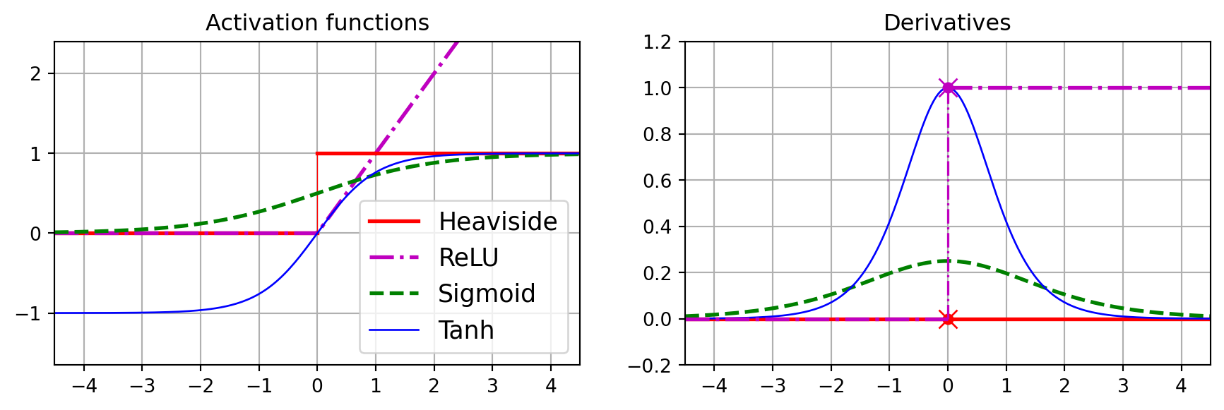
plt.plot([-max_z, 0], [0, 0], "r-", linewidth=2, label="Heaviside")
plt.plot(z, relu(z), "m-.", linewidth=2, label="ReLU")
plt.plot([0, 0], [0, 1], "r-", linewidth=0.5)
plt.plot([0, max_z], [1, 1], "r-", linewidth=2)
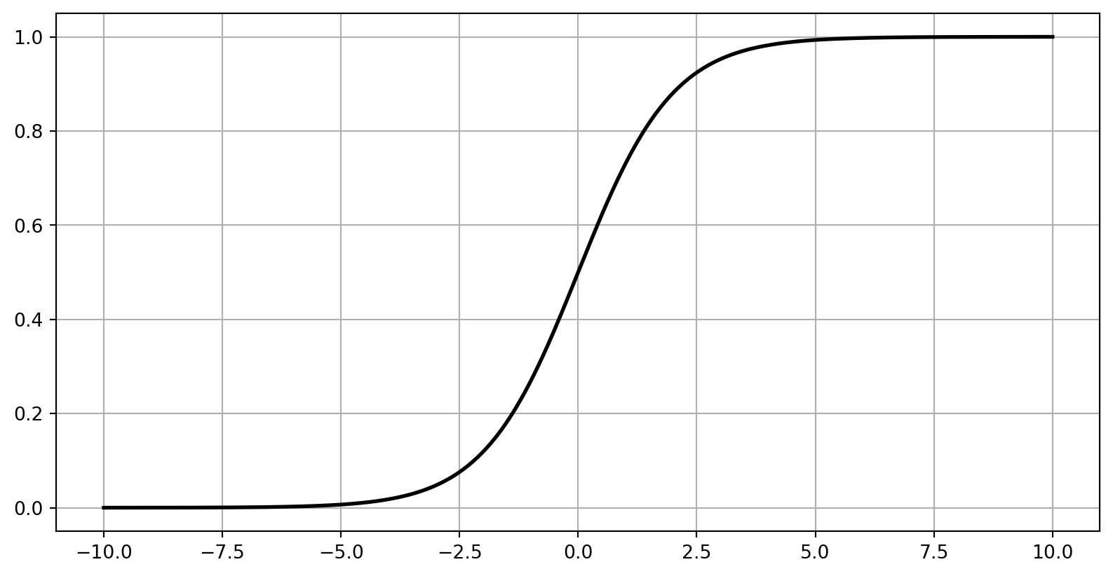
plt.plot(z, sigmoid(z), "g--", linewidth=2, label="Sigmoid")
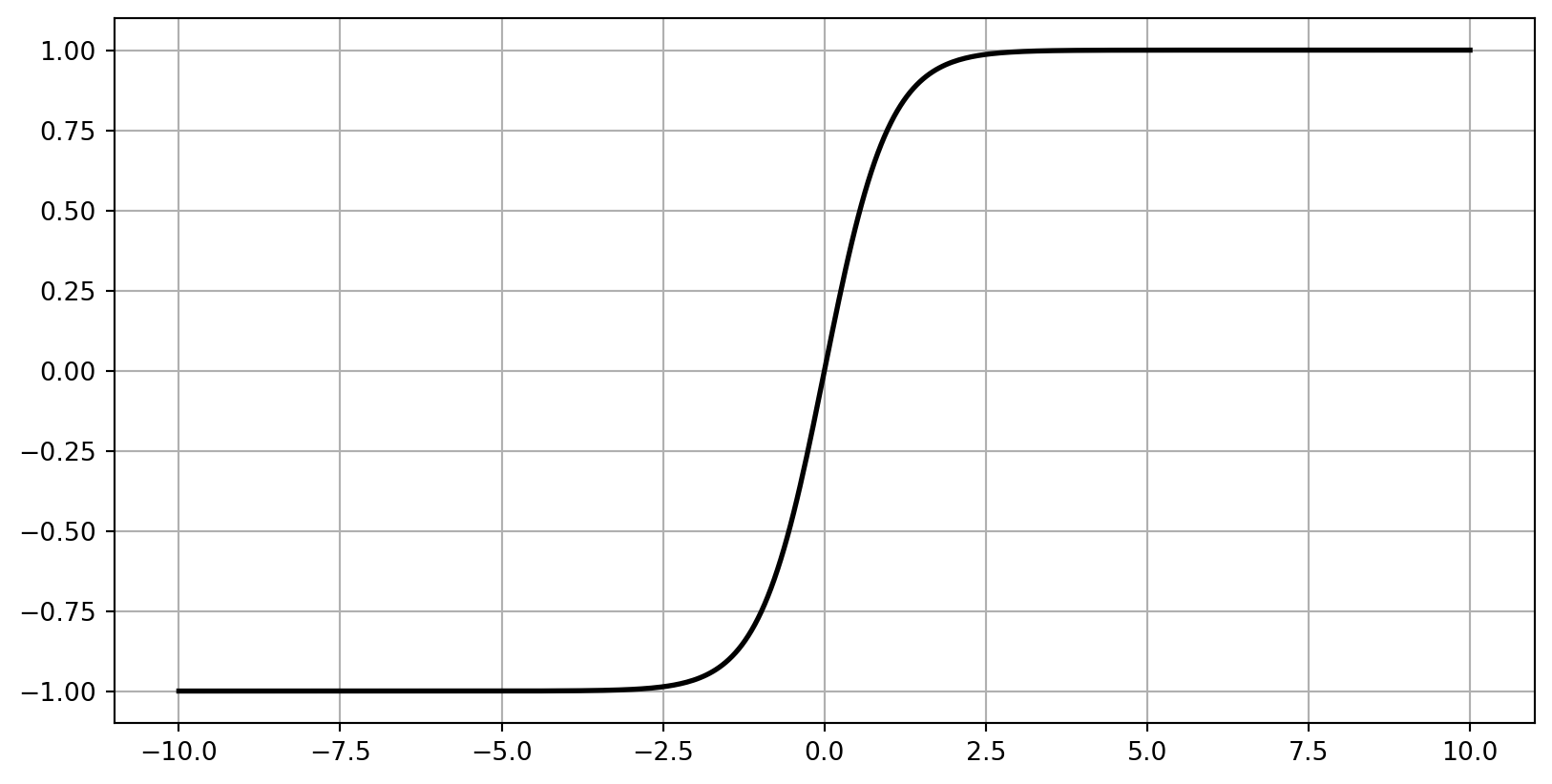
plt.plot(z, np.tanh(z), "b-", linewidth=1, label="Tanh")
plt.grid(True)
plt.title("Activation functions")
plt.axis([-max_z, max_z, -1.65, 2.4])
plt.gca().set_yticks([-1, 0, 1, 2])
plt.legend(loc="lower right", fontsize=13)

plt.subplot(122)
plt.plot(z, derivative(np.sign, z), "r-", linewidth=2, label="Heaviside")
plt.plot(0, 0, "ro", markersize=5)
plt.plot(0, 0, "rx", markersize=10)
plt.plot(z, derivative(sigmoid, z), "g--", linewidth=2, label="Sigmoid")
plt.plot(z, derivative(np.tanh, z), "b-", linewidth=1, label="Tanh")
plt.plot([-max_z, 0], [0, 0], "m-.", linewidth=2)
plt.plot([0, max_z], [1, 1], "m-.", linewidth=2)
plt.plot([0, 0], [0, 1], "m-.", linewidth=1.2)
plt.plot(0, 1, "mo", markersize=5)
plt.plot(0, 1, "mx", markersize=10)
plt.grid(True)
plt.title("Derivatives")
plt.axis([-max_z, max_z, -0.2, 1.2])

plt.show()

Universal Approximation

Definition

The universal approximation theorem (UAT) states that a feedforward neural network with a single hidden layer containing a finite number of neurons can approximate any continuous function on a compact subset of \(\mathbb{R}^n\), given appropriate weights and activation functions.

Single Hidden Layer

\[ y = \sum_{i=1}^N \alpha_i \sigma(w_{1,i} x + b_i) \]

Effect of Varying w

Code

def logistic(x, w, b):
    """Compute the logistic function with parameters w and b."""
    return 1 / (1 + np.exp(-(w * x + b)))

# Define a range for x values.
x = np.linspace(-10, 10, 400)

# Plot 1: Varying w (steepness) with b fixed at 0.
plt.figure(figsize=(6,4))
w_values = [0.5, 1, 2, 5]  # different steepness values
b = 0  # fixed bias

for w in w_values:
    plt.plot(x, logistic(x, w, b), label=f'w = {w}, b = {b}')
plt.title('Effect of Varying w (with b = 0)')
plt.xlabel('x')
plt.ylabel(r'$\sigma(wx+b)$')
plt.legend()
plt.grid(True)

plt.show()

Effect of Varying b

Code

# Plot 2: Varying b (horizontal shift) with w fixed at 1.
plt.figure(figsize=(6,4))
w = 1  # fixed steepness
b_values = [-5, -2, 0, 2, 5]  # different bias values

for b in b_values:
    plt.plot(x, logistic(x, w, b), label=f'w = {w}, b = {b}')
plt.title('Effect of Varying b (with w = 1)')
plt.xlabel('x')
plt.ylabel(r'$\sigma(wx+b)$')
plt.legend()
plt.grid(True)

plt.show()

Effect of Varying w

Code

def relu(x, w, b):
    """Compute the ReLU activation with parameters w and b."""
    return np.maximum(0, w * x + b)

# Define a range for x values.
x = np.linspace(-10, 10, 400)

# Plot 1: Varying w (scaling) with b fixed at 0.
plt.figure(figsize=(6,4))
w_values = [0.5, 1, 2, 5]  # different scaling values
b = 0  # fixed bias

for w in w_values:
    plt.plot(x, relu(x, w, b), label=f'w = {w}, b = {b}')
plt.title('Effect of Varying w (with b = 0) on ReLU Activation')
plt.xlabel('x')
plt.ylabel('ReLU(wx+b)')
plt.legend()
plt.grid(True)

plt.show()

Effect of Varying b

Code

# Plot 2: Varying b (horizontal shift) with w fixed at 1.
plt.figure(figsize=(6,4))
w = 1  # fixed scaling
b_values = [-5, -2, 0, 2, 5]  # different bias values

for b in b_values:
    plt.plot(x, relu(x, w, b), label=f'w = {w}, b = {b}')
plt.title('Effect of Varying b (with w = 1) on ReLU Activation')
plt.xlabel('x')
plt.ylabel('ReLU(wx+b)')
plt.legend()
plt.grid(True)

plt.show()

Single Hidden Layer

\[ y = \sum_{i=1}^N \alpha_i \sigma(w_{1,i} x + b_i) \]

Demonstration with code

# Defining the function to be approximated

def f(x):
  return 2 * x**3 + 4 * x**2 - 5 * x + 1

# Generating a dataset, x in [-4,2), f(x) as above

X = 6 * np.random.rand(1000, 1) - 4

y = f(X.flatten())

Increasing the number of neurons

from sklearn.neural_network import MLPRegressor
from sklearn.model_selection import train_test_split

X_train, X_valid, y_train, y_valid = train_test_split(X, y, test_size=0.1, random_state=42)

models = []

sizes = [1, 2, 5, 10, 100]

for i, n in enumerate(sizes):

  models.append(MLPRegressor(hidden_layer_sizes=[n], max_iter=5000, random_state=42))

  models[i].fit(X_train, y_train)

Increasing the number of neurons

Code

# Create a colormap
colors = plt.colormaps['cool'].resampled(len(sizes))

X_valid = np.sort(X_valid,axis=0)

for i, n in enumerate(sizes):

  y_pred = models[i].predict(X_valid)

  plt.plot(X_valid, y_pred, "-", color=colors(i), label="Number of neurons = {}".format(n))

y_true = f(X_valid)
plt.plot(X_valid, y_true, "r.", label='Actual')

plt.legend()
plt.show()

Increasing the number of neurons

Code

for i, n in enumerate(sizes):

  plt.plot(models[i].loss_curve_, "-", color=colors(i), label="Number of neurons = {}".format(n))

plt.title('MLPRegressor Loss Curves')
plt.xlabel('Iterations')
plt.ylabel('Loss')

plt.legend()
plt.show()

Universal Approximation

Let’s code

Frameworks

PyTorch and TensorFlow are the leading platforms for deep learning.

PyTorch has gained considerable traction in the research community. Initially developed by Meta AI, it is now part of the Linux Foundation.
TensorFlow, created by Google, is widely adopted in industry for deploying models in production environments.

Keras

Keras is a high-level API designed to build, train, evaluate, and execute models across various backends, including PyTorch, TensorFlow, and JAX, Google’s high-performance platform.

Fashion-MNIST dataset

“Fashion-MNIST is a dataset of Zalando’s article images—consisting of a training set of 60,000 examples and a test set of 10,000 examples. Each example is a 28x28 grayscale image, associated with a label from 10 classes.”

Loading

import tensorflow as tf

fashion_mnist = tf.keras.datasets.fashion_mnist

(X_train_full, y_train_full), (X_test, y_test) = fashion_mnist.load_data()

X_train, y_train = X_train_full[:-5000], y_train_full[:-5000]
X_valid, y_valid = X_train_full[-5000:], y_train_full[-5000:]

Exploration

X_train.shape

(55000, 28, 28)

X_train.dtype

dtype('uint8')

Transforming the pixel intensities from integers in the range 0 to 255 to floats in the range 0 to 1.

X_train = X_train / 255.0
X_valid = X_valid / 255.0

What are these images anyway!

plt.figure(figsize=(2, 2))
plt.imshow(X_train[0], cmap="binary")
plt.axis('off')
plt.show()

y_train

array([9, 0, 0, ..., 9, 0, 2], shape=(55000,), dtype=uint8)

Since the labels are integers, 0 to 9. Class names will become handy.

class_names = ["T-shirt/top", "Trouser", "Pullover", "Dress", "Coat",
               "Sandal", "Shirt", "Sneaker", "Bag", "Ankle boot"]

First 40 images

n_rows = 4
n_cols = 10
plt.figure(figsize=(n_cols * 1.2, n_rows * 1.2))
for row in range(n_rows):
    for col in range(n_cols):
        index = n_cols * row + col
        plt.subplot(n_rows, n_cols, index + 1)
        plt.imshow(X_train[index], cmap="binary", interpolation="nearest")
        plt.axis('off')
        plt.title(class_names[y_train[index]])
plt.subplots_adjust(wspace=0.2, hspace=0.5)
plt.show()

First 40 images

Creating a model

tf.random.set_seed(42)

model = tf.keras.Sequential()

model.add(tf.keras.layers.InputLayer(shape=[28, 28]))
model.add(tf.keras.layers.Flatten())
model.add(tf.keras.layers.Dense(300, activation="relu"))
model.add(tf.keras.layers.Dense(100, activation="relu"))
model.add(tf.keras.layers.Dense(10, activation="softmax"))

`model.summary()`

Code

model.summary()

Model: "sequential"

┏━━━━━━━━━━━━━━━━━━━━━━━━━━━━━━━━━┳━━━━━━━━━━━━━━━━━━━━━━━━┳━━━━━━━━━━━━━━━┓
┃ Layer (type)                    ┃ Output Shape           ┃       Param # ┃
┡━━━━━━━━━━━━━━━━━━━━━━━━━━━━━━━━━╇━━━━━━━━━━━━━━━━━━━━━━━━╇━━━━━━━━━━━━━━━┩
│ flatten (Flatten)               │ (None, 784)            │             0 │
├─────────────────────────────────┼────────────────────────┼───────────────┤
│ dense (Dense)                   │ (None, 300)            │       235,500 │
├─────────────────────────────────┼────────────────────────┼───────────────┤
│ dense_1 (Dense)                 │ (None, 100)            │        30,100 │
├─────────────────────────────────┼────────────────────────┼───────────────┤
│ dense_2 (Dense)                 │ (None, 10)             │         1,010 │
└─────────────────────────────────┴────────────────────────┴───────────────┘

 Total params: 266,610 (1.02 MB)

 Trainable params: 266,610 (1.02 MB)

 Non-trainable params: 0 (0.00 B)

Creating a model (alternative)

Code

# extra code – clear the session to reset the name counters
tf.keras.backend.clear_session()
tf.random.set_seed(42)

model = tf.keras.Sequential([
    tf.keras.Input(shape=(28, 28)),
    tf.keras.layers.Flatten(),
    tf.keras.layers.Dense(300, activation="relu"),
    tf.keras.layers.Dense(100, activation="relu"),
    tf.keras.layers.Dense(10, activation="softmax")
])

`model.summary()`

Code

model.summary()

Model: "sequential"

┏━━━━━━━━━━━━━━━━━━━━━━━━━━━━━━━━━┳━━━━━━━━━━━━━━━━━━━━━━━━┳━━━━━━━━━━━━━━━┓
┃ Layer (type)                    ┃ Output Shape           ┃       Param # ┃
┡━━━━━━━━━━━━━━━━━━━━━━━━━━━━━━━━━╇━━━━━━━━━━━━━━━━━━━━━━━━╇━━━━━━━━━━━━━━━┩
│ flatten (Flatten)               │ (None, 784)            │             0 │
├─────────────────────────────────┼────────────────────────┼───────────────┤
│ dense (Dense)                   │ (None, 300)            │       235,500 │
├─────────────────────────────────┼────────────────────────┼───────────────┤
│ dense_1 (Dense)                 │ (None, 100)            │        30,100 │
├─────────────────────────────────┼────────────────────────┼───────────────┤
│ dense_2 (Dense)                 │ (None, 10)             │         1,010 │
└─────────────────────────────────┴────────────────────────┴───────────────┘

 Total params: 266,610 (1.02 MB)

 Trainable params: 266,610 (1.02 MB)

 Non-trainable params: 0 (0.00 B)

Compiling the model

model.compile(loss="sparse_categorical_crossentropy",
              optimizer="sgd",
              metrics=["accuracy"])

Training the model

history = model.fit(X_train, y_train, epochs=30,
                    validation_data=(X_valid, y_valid))

Epoch 1/30


   1/1719 ━━━━━━━━━━━━━━━━━━━━ 6:33 229ms/step - accuracy: 0.0938 - loss: 2.3631

  59/1719 ━━━━━━━━━━━━━━━━━━━━ 1s 871us/step - accuracy: 0.2212 - loss: 2.1282  

 122/1719 ━━━━━━━━━━━━━━━━━━━━ 1s 835us/step - accuracy: 0.3330 - loss: 1.9682

 186/1719 ━━━━━━━━━━━━━━━━━━━━ 1s 819us/step - accuracy: 0.3990 - loss: 1.8385

 250/1719 ━━━━━━━━━━━━━━━━━━━━ 1s 812us/step - accuracy: 0.4440 - loss: 1.7337

 313/1719 ━━━━━━━━━━━━━━━━━━━━ 1s 809us/step - accuracy: 0.4758 - loss: 1.6497

 380/1719 ━━━━━━━━━━━━━━━━━━━━ 1s 799us/step - accuracy: 0.5022 - loss: 1.5750

 444/1719 ━━━━━━━━━━━━━━━━━━━━ 1s 797us/step - accuracy: 0.5224 - loss: 1.5150

 509/1719 ━━━━━━━━━━━━━━━━━━━━ 0s 795us/step - accuracy: 0.5396 - loss: 1.4625

 574/1719 ━━━━━━━━━━━━━━━━━━━━ 0s 793us/step - accuracy: 0.5542 - loss: 1.4167

 637/1719 ━━━━━━━━━━━━━━━━━━━━ 0s 794us/step - accuracy: 0.5666 - loss: 1.3774

 702/1719 ━━━━━━━━━━━━━━━━━━━━ 0s 792us/step - accuracy: 0.5780 - loss: 1.3411

 766/1719 ━━━━━━━━━━━━━━━━━━━━ 0s 792us/step - accuracy: 0.5879 - loss: 1.3091

 829/1719 ━━━━━━━━━━━━━━━━━━━━ 0s 792us/step - accuracy: 0.5968 - loss: 1.2804

 893/1719 ━━━━━━━━━━━━━━━━━━━━ 0s 792us/step - accuracy: 0.6049 - loss: 1.2537

 957/1719 ━━━━━━━━━━━━━━━━━━━━ 0s 791us/step - accuracy: 0.6124 - loss: 1.2291

1021/1719 ━━━━━━━━━━━━━━━━━━━━ 0s 792us/step - accuracy: 0.6193 - loss: 1.2064

1085/1719 ━━━━━━━━━━━━━━━━━━━━ 0s 791us/step - accuracy: 0.6256 - loss: 1.1853

1149/1719 ━━━━━━━━━━━━━━━━━━━━ 0s 791us/step - accuracy: 0.6315 - loss: 1.1658

1212/1719 ━━━━━━━━━━━━━━━━━━━━ 0s 791us/step - accuracy: 0.6369 - loss: 1.1479

1275/1719 ━━━━━━━━━━━━━━━━━━━━ 0s 792us/step - accuracy: 0.6419 - loss: 1.1312

1340/1719 ━━━━━━━━━━━━━━━━━━━━ 0s 791us/step - accuracy: 0.6467 - loss: 1.1149

1406/1719 ━━━━━━━━━━━━━━━━━━━━ 0s 789us/step - accuracy: 0.6514 - loss: 1.0994

1470/1719 ━━━━━━━━━━━━━━━━━━━━ 0s 790us/step - accuracy: 0.6556 - loss: 1.0852

1533/1719 ━━━━━━━━━━━━━━━━━━━━ 0s 790us/step - accuracy: 0.6595 - loss: 1.0719

1598/1719 ━━━━━━━━━━━━━━━━━━━━ 0s 789us/step - accuracy: 0.6634 - loss: 1.0590

1661/1719 ━━━━━━━━━━━━━━━━━━━━ 0s 790us/step - accuracy: 0.6669 - loss: 1.0471

1719/1719 ━━━━━━━━━━━━━━━━━━━━ 2s 898us/step - accuracy: 0.7589 - loss: 0.7349 - val_accuracy: 0.8230 - val_loss: 0.5102

Epoch 2/30


   1/1719 ━━━━━━━━━━━━━━━━━━━━ 15s 9ms/step - accuracy: 0.8438 - loss: 0.4986

  69/1719 ━━━━━━━━━━━━━━━━━━━━ 1s 743us/step - accuracy: 0.8427 - loss: 0.4945

 138/1719 ━━━━━━━━━━━━━━━━━━━━ 1s 736us/step - accuracy: 0.8324 - loss: 0.5131

 208/1719 ━━━━━━━━━━━━━━━━━━━━ 1s 729us/step - accuracy: 0.8281 - loss: 0.5191

 277/1719 ━━━━━━━━━━━━━━━━━━━━ 1s 729us/step - accuracy: 0.8267 - loss: 0.5204

 346/1719 ━━━━━━━━━━━━━━━━━━━━ 0s 728us/step - accuracy: 0.8257 - loss: 0.5209

 415/1719 ━━━━━━━━━━━━━━━━━━━━ 0s 728us/step - accuracy: 0.8251 - loss: 0.5212

 485/1719 ━━━━━━━━━━━━━━━━━━━━ 0s 726us/step - accuracy: 0.8245 - loss: 0.5211

 556/1719 ━━━━━━━━━━━━━━━━━━━━ 0s 725us/step - accuracy: 0.8241 - loss: 0.5208

 627/1719 ━━━━━━━━━━━━━━━━━━━━ 0s 723us/step - accuracy: 0.8240 - loss: 0.5203

 697/1719 ━━━━━━━━━━━━━━━━━━━━ 0s 723us/step - accuracy: 0.8239 - loss: 0.5196

 768/1719 ━━━━━━━━━━━━━━━━━━━━ 0s 721us/step - accuracy: 0.8240 - loss: 0.5190

 840/1719 ━━━━━━━━━━━━━━━━━━━━ 0s 720us/step - accuracy: 0.8241 - loss: 0.5182

 911/1719 ━━━━━━━━━━━━━━━━━━━━ 0s 719us/step - accuracy: 0.8242 - loss: 0.5175

 982/1719 ━━━━━━━━━━━━━━━━━━━━ 0s 718us/step - accuracy: 0.8244 - loss: 0.5165

1051/1719 ━━━━━━━━━━━━━━━━━━━━ 0s 719us/step - accuracy: 0.8246 - loss: 0.5155

1122/1719 ━━━━━━━━━━━━━━━━━━━━ 0s 718us/step - accuracy: 0.8248 - loss: 0.5145

1193/1719 ━━━━━━━━━━━━━━━━━━━━ 0s 717us/step - accuracy: 0.8249 - loss: 0.5136

1263/1719 ━━━━━━━━━━━━━━━━━━━━ 0s 717us/step - accuracy: 0.8251 - loss: 0.5127

1334/1719 ━━━━━━━━━━━━━━━━━━━━ 0s 717us/step - accuracy: 0.8253 - loss: 0.5119

1404/1719 ━━━━━━━━━━━━━━━━━━━━ 0s 717us/step - accuracy: 0.8255 - loss: 0.5110

1475/1719 ━━━━━━━━━━━━━━━━━━━━ 0s 717us/step - accuracy: 0.8257 - loss: 0.5101

1545/1719 ━━━━━━━━━━━━━━━━━━━━ 0s 717us/step - accuracy: 0.8259 - loss: 0.5093

1617/1719 ━━━━━━━━━━━━━━━━━━━━ 0s 716us/step - accuracy: 0.8262 - loss: 0.5084

1687/1719 ━━━━━━━━━━━━━━━━━━━━ 0s 716us/step - accuracy: 0.8263 - loss: 0.5076

1719/1719 ━━━━━━━━━━━━━━━━━━━━ 1s 765us/step - accuracy: 0.8303 - loss: 0.4885 - val_accuracy: 0.8364 - val_loss: 0.4572

Epoch 3/30


   1/1719 ━━━━━━━━━━━━━━━━━━━━ 14s 9ms/step - accuracy: 0.8438 - loss: 0.4497

  73/1719 ━━━━━━━━━━━━━━━━━━━━ 1s 702us/step - accuracy: 0.8548 - loss: 0.4311

 143/1719 ━━━━━━━━━━━━━━━━━━━━ 1s 712us/step - accuracy: 0.8470 - loss: 0.4492

 215/1719 ━━━━━━━━━━━━━━━━━━━━ 1s 709us/step - accuracy: 0.8441 - loss: 0.4551

 285/1719 ━━━━━━━━━━━━━━━━━━━━ 1s 711us/step - accuracy: 0.8431 - loss: 0.4569

 357/1719 ━━━━━━━━━━━━━━━━━━━━ 0s 709us/step - accuracy: 0.8422 - loss: 0.4579

 427/1719 ━━━━━━━━━━━━━━━━━━━━ 0s 710us/step - accuracy: 0.8414 - loss: 0.4588

 499/1719 ━━━━━━━━━━━━━━━━━━━━ 0s 709us/step - accuracy: 0.8408 - loss: 0.4592

 572/1719 ━━━━━━━━━━━━━━━━━━━━ 0s 707us/step - accuracy: 0.8405 - loss: 0.4595

 644/1719 ━━━━━━━━━━━━━━━━━━━━ 0s 706us/step - accuracy: 0.8404 - loss: 0.4594

 716/1719 ━━━━━━━━━━━━━━━━━━━━ 0s 705us/step - accuracy: 0.8405 - loss: 0.4593

 789/1719 ━━━━━━━━━━━━━━━━━━━━ 0s 704us/step - accuracy: 0.8405 - loss: 0.4592

 861/1719 ━━━━━━━━━━━━━━━━━━━━ 0s 704us/step - accuracy: 0.8407 - loss: 0.4589

 933/1719 ━━━━━━━━━━━━━━━━━━━━ 0s 704us/step - accuracy: 0.8408 - loss: 0.4586

1005/1719 ━━━━━━━━━━━━━━━━━━━━ 0s 704us/step - accuracy: 0.8410 - loss: 0.4581

1077/1719 ━━━━━━━━━━━━━━━━━━━━ 0s 703us/step - accuracy: 0.8411 - loss: 0.4576

1148/1719 ━━━━━━━━━━━━━━━━━━━━ 0s 704us/step - accuracy: 0.8413 - loss: 0.4571

1218/1719 ━━━━━━━━━━━━━━━━━━━━ 0s 704us/step - accuracy: 0.8414 - loss: 0.4566

1290/1719 ━━━━━━━━━━━━━━━━━━━━ 0s 704us/step - accuracy: 0.8416 - loss: 0.4562

1354/1719 ━━━━━━━━━━━━━━━━━━━━ 0s 708us/step - accuracy: 0.8417 - loss: 0.4557

1420/1719 ━━━━━━━━━━━━━━━━━━━━ 0s 711us/step - accuracy: 0.8419 - loss: 0.4552

1485/1719 ━━━━━━━━━━━━━━━━━━━━ 0s 714us/step - accuracy: 0.8420 - loss: 0.4548

1549/1719 ━━━━━━━━━━━━━━━━━━━━ 0s 716us/step - accuracy: 0.8422 - loss: 0.4544

1613/1719 ━━━━━━━━━━━━━━━━━━━━ 0s 719us/step - accuracy: 0.8423 - loss: 0.4539

1678/1719 ━━━━━━━━━━━━━━━━━━━━ 0s 721us/step - accuracy: 0.8424 - loss: 0.4535

1719/1719 ━━━━━━━━━━━━━━━━━━━━ 1s 773us/step - accuracy: 0.8450 - loss: 0.4428 - val_accuracy: 0.8446 - val_loss: 0.4312

Epoch 4/30


   1/1719 ━━━━━━━━━━━━━━━━━━━━ 15s 9ms/step - accuracy: 0.8750 - loss: 0.4299

  65/1719 ━━━━━━━━━━━━━━━━━━━━ 1s 786us/step - accuracy: 0.8693 - loss: 0.3958

 131/1719 ━━━━━━━━━━━━━━━━━━━━ 1s 776us/step - accuracy: 0.8621 - loss: 0.4125

 196/1719 ━━━━━━━━━━━━━━━━━━━━ 1s 777us/step - accuracy: 0.8584 - loss: 0.4203

 264/1719 ━━━━━━━━━━━━━━━━━━━━ 1s 767us/step - accuracy: 0.8568 - loss: 0.4226

 330/1719 ━━━━━━━━━━━━━━━━━━━━ 1s 767us/step - accuracy: 0.8556 - loss: 0.4241

 398/1719 ━━━━━━━━━━━━━━━━━━━━ 1s 763us/step - accuracy: 0.8546 - loss: 0.4253

 463/1719 ━━━━━━━━━━━━━━━━━━━━ 0s 764us/step - accuracy: 0.8539 - loss: 0.4261

 530/1719 ━━━━━━━━━━━━━━━━━━━━ 0s 763us/step - accuracy: 0.8533 - loss: 0.4266

 597/1719 ━━━━━━━━━━━━━━━━━━━━ 0s 762us/step - accuracy: 0.8529 - loss: 0.4269

 662/1719 ━━━━━━━━━━━━━━━━━━━━ 0s 763us/step - accuracy: 0.8528 - loss: 0.4269

 727/1719 ━━━━━━━━━━━━━━━━━━━━ 0s 765us/step - accuracy: 0.8527 - loss: 0.4270

 792/1719 ━━━━━━━━━━━━━━━━━━━━ 0s 766us/step - accuracy: 0.8526 - loss: 0.4270

 857/1719 ━━━━━━━━━━━━━━━━━━━━ 0s 767us/step - accuracy: 0.8526 - loss: 0.4269

 924/1719 ━━━━━━━━━━━━━━━━━━━━ 0s 766us/step - accuracy: 0.8526 - loss: 0.4268

 989/1719 ━━━━━━━━━━━━━━━━━━━━ 0s 767us/step - accuracy: 0.8526 - loss: 0.4265

1054/1719 ━━━━━━━━━━━━━━━━━━━━ 0s 767us/step - accuracy: 0.8527 - loss: 0.4262

1119/1719 ━━━━━━━━━━━━━━━━━━━━ 0s 767us/step - accuracy: 0.8527 - loss: 0.4258

1185/1719 ━━━━━━━━━━━━━━━━━━━━ 0s 767us/step - accuracy: 0.8528 - loss: 0.4255

1250/1719 ━━━━━━━━━━━━━━━━━━━━ 0s 767us/step - accuracy: 0.8528 - loss: 0.4252

1314/1719 ━━━━━━━━━━━━━━━━━━━━ 0s 768us/step - accuracy: 0.8528 - loss: 0.4249

1379/1719 ━━━━━━━━━━━━━━━━━━━━ 0s 769us/step - accuracy: 0.8529 - loss: 0.4246

1445/1719 ━━━━━━━━━━━━━━━━━━━━ 0s 768us/step - accuracy: 0.8529 - loss: 0.4242

1511/1719 ━━━━━━━━━━━━━━━━━━━━ 0s 768us/step - accuracy: 0.8530 - loss: 0.4239

1576/1719 ━━━━━━━━━━━━━━━━━━━━ 0s 769us/step - accuracy: 0.8531 - loss: 0.4235

1642/1719 ━━━━━━━━━━━━━━━━━━━━ 0s 769us/step - accuracy: 0.8531 - loss: 0.4232

1708/1719 ━━━━━━━━━━━━━━━━━━━━ 0s 768us/step - accuracy: 0.8532 - loss: 0.4229

1719/1719 ━━━━━━━━━━━━━━━━━━━━ 1s 824us/step - accuracy: 0.8542 - loss: 0.4151 - val_accuracy: 0.8506 - val_loss: 0.4143

Epoch 5/30


   1/1719 ━━━━━━━━━━━━━━━━━━━━ 16s 10ms/step - accuracy: 0.8750 - loss: 0.4091

  66/1719 ━━━━━━━━━━━━━━━━━━━━ 1s 779us/step - accuracy: 0.8704 - loss: 0.3721

 132/1719 ━━━━━━━━━━━━━━━━━━━━ 1s 768us/step - accuracy: 0.8657 - loss: 0.3886

 199/1719 ━━━━━━━━━━━━━━━━━━━━ 1s 762us/step - accuracy: 0.8628 - loss: 0.3968

 263/1719 ━━━━━━━━━━━━━━━━━━━━ 1s 767us/step - accuracy: 0.8618 - loss: 0.3991

 329/1719 ━━━━━━━━━━━━━━━━━━━━ 1s 767us/step - accuracy: 0.8607 - loss: 0.4008

 395/1719 ━━━━━━━━━━━━━━━━━━━━ 1s 766us/step - accuracy: 0.8600 - loss: 0.4022

 461/1719 ━━━━━━━━━━━━━━━━━━━━ 0s 765us/step - accuracy: 0.8595 - loss: 0.4031

 527/1719 ━━━━━━━━━━━━━━━━━━━━ 0s 765us/step - accuracy: 0.8591 - loss: 0.4038

 592/1719 ━━━━━━━━━━━━━━━━━━━━ 0s 767us/step - accuracy: 0.8589 - loss: 0.4041

 663/1719 ━━━━━━━━━━━━━━━━━━━━ 0s 761us/step - accuracy: 0.8589 - loss: 0.4042

 734/1719 ━━━━━━━━━━━━━━━━━━━━ 0s 755us/step - accuracy: 0.8590 - loss: 0.4043

 803/1719 ━━━━━━━━━━━━━━━━━━━━ 0s 754us/step - accuracy: 0.8590 - loss: 0.4044

 868/1719 ━━━━━━━━━━━━━━━━━━━━ 0s 755us/step - accuracy: 0.8590 - loss: 0.4044

 933/1719 ━━━━━━━━━━━━━━━━━━━━ 0s 756us/step - accuracy: 0.8591 - loss: 0.4044

 999/1719 ━━━━━━━━━━━━━━━━━━━━ 0s 756us/step - accuracy: 0.8592 - loss: 0.4042

1066/1719 ━━━━━━━━━━━━━━━━━━━━ 0s 756us/step - accuracy: 0.8593 - loss: 0.4039

1131/1719 ━━━━━━━━━━━━━━━━━━━━ 0s 757us/step - accuracy: 0.8594 - loss: 0.4036

1198/1719 ━━━━━━━━━━━━━━━━━━━━ 0s 757us/step - accuracy: 0.8594 - loss: 0.4033

1264/1719 ━━━━━━━━━━━━━━━━━━━━ 0s 757us/step - accuracy: 0.8595 - loss: 0.4031

1330/1719 ━━━━━━━━━━━━━━━━━━━━ 0s 757us/step - accuracy: 0.8596 - loss: 0.4029

1395/1719 ━━━━━━━━━━━━━━━━━━━━ 0s 758us/step - accuracy: 0.8596 - loss: 0.4026

1461/1719 ━━━━━━━━━━━━━━━━━━━━ 0s 758us/step - accuracy: 0.8597 - loss: 0.4023

1529/1719 ━━━━━━━━━━━━━━━━━━━━ 0s 758us/step - accuracy: 0.8598 - loss: 0.4020

1596/1719 ━━━━━━━━━━━━━━━━━━━━ 0s 757us/step - accuracy: 0.8598 - loss: 0.4017

1662/1719 ━━━━━━━━━━━━━━━━━━━━ 0s 758us/step - accuracy: 0.8599 - loss: 0.4014

1719/1719 ━━━━━━━━━━━━━━━━━━━━ 1s 810us/step - accuracy: 0.8609 - loss: 0.3949 - val_accuracy: 0.8572 - val_loss: 0.4024

Epoch 6/30


   1/1719 ━━━━━━━━━━━━━━━━━━━━ 16s 9ms/step - accuracy: 0.8750 - loss: 0.3935

  66/1719 ━━━━━━━━━━━━━━━━━━━━ 1s 780us/step - accuracy: 0.8779 - loss: 0.3546

 132/1719 ━━━━━━━━━━━━━━━━━━━━ 1s 772us/step - accuracy: 0.8728 - loss: 0.3705

 198/1719 ━━━━━━━━━━━━━━━━━━━━ 1s 770us/step - accuracy: 0.8698 - loss: 0.3786

 264/1719 ━━━━━━━━━━━━━━━━━━━━ 1s 770us/step - accuracy: 0.8687 - loss: 0.3811

 329/1719 ━━━━━━━━━━━━━━━━━━━━ 1s 770us/step - accuracy: 0.8676 - loss: 0.3829

 395/1719 ━━━━━━━━━━━━━━━━━━━━ 1s 768us/step - accuracy: 0.8667 - loss: 0.3843

 461/1719 ━━━━━━━━━━━━━━━━━━━━ 0s 768us/step - accuracy: 0.8661 - loss: 0.3852

 527/1719 ━━━━━━━━━━━━━━━━━━━━ 0s 768us/step - accuracy: 0.8656 - loss: 0.3859

 594/1719 ━━━━━━━━━━━━━━━━━━━━ 0s 766us/step - accuracy: 0.8653 - loss: 0.3864

 661/1719 ━━━━━━━━━━━━━━━━━━━━ 0s 764us/step - accuracy: 0.8652 - loss: 0.3865

 727/1719 ━━━━━━━━━━━━━━━━━━━━ 0s 764us/step - accuracy: 0.8652 - loss: 0.3866

 793/1719 ━━━━━━━━━━━━━━━━━━━━ 0s 764us/step - accuracy: 0.8651 - loss: 0.3867

 859/1719 ━━━━━━━━━━━━━━━━━━━━ 0s 764us/step - accuracy: 0.8651 - loss: 0.3867

 926/1719 ━━━━━━━━━━━━━━━━━━━━ 0s 764us/step - accuracy: 0.8651 - loss: 0.3867

 993/1719 ━━━━━━━━━━━━━━━━━━━━ 0s 763us/step - accuracy: 0.8651 - loss: 0.3866

1061/1719 ━━━━━━━━━━━━━━━━━━━━ 0s 762us/step - accuracy: 0.8652 - loss: 0.3864

1126/1719 ━━━━━━━━━━━━━━━━━━━━ 0s 762us/step - accuracy: 0.8652 - loss: 0.3861

1191/1719 ━━━━━━━━━━━━━━━━━━━━ 0s 763us/step - accuracy: 0.8653 - loss: 0.3859

1257/1719 ━━━━━━━━━━━━━━━━━━━━ 0s 763us/step - accuracy: 0.8653 - loss: 0.3857

1323/1719 ━━━━━━━━━━━━━━━━━━━━ 0s 763us/step - accuracy: 0.8654 - loss: 0.3855

1389/1719 ━━━━━━━━━━━━━━━━━━━━ 0s 763us/step - accuracy: 0.8654 - loss: 0.3852

1455/1719 ━━━━━━━━━━━━━━━━━━━━ 0s 763us/step - accuracy: 0.8655 - loss: 0.3850

1521/1719 ━━━━━━━━━━━━━━━━━━━━ 0s 763us/step - accuracy: 0.8656 - loss: 0.3847

1587/1719 ━━━━━━━━━━━━━━━━━━━━ 0s 763us/step - accuracy: 0.8656 - loss: 0.3845

1653/1719 ━━━━━━━━━━━━━━━━━━━━ 0s 763us/step - accuracy: 0.8656 - loss: 0.3842

1719/1719 ━━━━━━━━━━━━━━━━━━━━ 0s 763us/step - accuracy: 0.8657 - loss: 0.3840

1719/1719 ━━━━━━━━━━━━━━━━━━━━ 1s 814us/step - accuracy: 0.8663 - loss: 0.3786 - val_accuracy: 0.8602 - val_loss: 0.3916

Epoch 7/30


   1/1719 ━━━━━━━━━━━━━━━━━━━━ 15s 9ms/step - accuracy: 0.8750 - loss: 0.3802

  70/1719 ━━━━━━━━━━━━━━━━━━━━ 1s 731us/step - accuracy: 0.8790 - loss: 0.3399

 140/1719 ━━━━━━━━━━━━━━━━━━━━ 1s 724us/step - accuracy: 0.8743 - loss: 0.3567

 209/1719 ━━━━━━━━━━━━━━━━━━━━ 1s 725us/step - accuracy: 0.8717 - loss: 0.3639

 279/1719 ━━━━━━━━━━━━━━━━━━━━ 1s 724us/step - accuracy: 0.8708 - loss: 0.3666

 346/1719 ━━━━━━━━━━━━━━━━━━━━ 1s 729us/step - accuracy: 0.8701 - loss: 0.3683

 409/1719 ━━━━━━━━━━━━━━━━━━━━ 0s 740us/step - accuracy: 0.8695 - loss: 0.3697

 474/1719 ━━━━━━━━━━━━━━━━━━━━ 0s 745us/step - accuracy: 0.8692 - loss: 0.3706

 539/1719 ━━━━━━━━━━━━━━━━━━━━ 0s 748us/step - accuracy: 0.8689 - loss: 0.3713

 605/1719 ━━━━━━━━━━━━━━━━━━━━ 0s 750us/step - accuracy: 0.8688 - loss: 0.3716

 670/1719 ━━━━━━━━━━━━━━━━━━━━ 0s 752us/step - accuracy: 0.8688 - loss: 0.3717

 737/1719 ━━━━━━━━━━━━━━━━━━━━ 0s 753us/step - accuracy: 0.8688 - loss: 0.3719

 803/1719 ━━━━━━━━━━━━━━━━━━━━ 0s 754us/step - accuracy: 0.8688 - loss: 0.3720

 868/1719 ━━━━━━━━━━━━━━━━━━━━ 0s 756us/step - accuracy: 0.8689 - loss: 0.3721

 934/1719 ━━━━━━━━━━━━━━━━━━━━ 0s 756us/step - accuracy: 0.8689 - loss: 0.3721

 999/1719 ━━━━━━━━━━━━━━━━━━━━ 0s 758us/step - accuracy: 0.8690 - loss: 0.3720

1066/1719 ━━━━━━━━━━━━━━━━━━━━ 0s 757us/step - accuracy: 0.8691 - loss: 0.3718

1134/1719 ━━━━━━━━━━━━━━━━━━━━ 0s 756us/step - accuracy: 0.8692 - loss: 0.3716

1200/1719 ━━━━━━━━━━━━━━━━━━━━ 0s 756us/step - accuracy: 0.8693 - loss: 0.3713

1266/1719 ━━━━━━━━━━━━━━━━━━━━ 0s 756us/step - accuracy: 0.8693 - loss: 0.3712

1331/1719 ━━━━━━━━━━━━━━━━━━━━ 0s 757us/step - accuracy: 0.8694 - loss: 0.3710

1398/1719 ━━━━━━━━━━━━━━━━━━━━ 0s 757us/step - accuracy: 0.8695 - loss: 0.3708

1465/1719 ━━━━━━━━━━━━━━━━━━━━ 0s 757us/step - accuracy: 0.8696 - loss: 0.3705

1534/1719 ━━━━━━━━━━━━━━━━━━━━ 0s 756us/step - accuracy: 0.8696 - loss: 0.3703

1602/1719 ━━━━━━━━━━━━━━━━━━━━ 0s 755us/step - accuracy: 0.8697 - loss: 0.3701

1670/1719 ━━━━━━━━━━━━━━━━━━━━ 0s 754us/step - accuracy: 0.8698 - loss: 0.3699

1719/1719 ━━━━━━━━━━━━━━━━━━━━ 1s 808us/step - accuracy: 0.8707 - loss: 0.3650 - val_accuracy: 0.8616 - val_loss: 0.3837

Epoch 8/30


   1/1719 ━━━━━━━━━━━━━━━━━━━━ 15s 9ms/step - accuracy: 0.8750 - loss: 0.3662

  67/1719 ━━━━━━━━━━━━━━━━━━━━ 1s 766us/step - accuracy: 0.8814 - loss: 0.3264

 135/1719 ━━━━━━━━━━━━━━━━━━━━ 1s 756us/step - accuracy: 0.8774 - loss: 0.3423

 200/1719 ━━━━━━━━━━━━━━━━━━━━ 1s 763us/step - accuracy: 0.8750 - loss: 0.3501

 266/1719 ━━━━━━━━━━━━━━━━━━━━ 1s 762us/step - accuracy: 0.8741 - loss: 0.3529

 328/1719 ━━━━━━━━━━━━━━━━━━━━ 1s 771us/step - accuracy: 0.8733 - loss: 0.3548

 390/1719 ━━━━━━━━━━━━━━━━━━━━ 1s 778us/step - accuracy: 0.8727 - loss: 0.3563

 453/1719 ━━━━━━━━━━━━━━━━━━━━ 0s 782us/step - accuracy: 0.8722 - loss: 0.3574

 517/1719 ━━━━━━━━━━━━━━━━━━━━ 0s 783us/step - accuracy: 0.8718 - loss: 0.3582

 580/1719 ━━━━━━━━━━━━━━━━━━━━ 0s 784us/step - accuracy: 0.8716 - loss: 0.3587

 644/1719 ━━━━━━━━━━━━━━━━━━━━ 0s 784us/step - accuracy: 0.8716 - loss: 0.3589

 709/1719 ━━━━━━━━━━━━━━━━━━━━ 0s 784us/step - accuracy: 0.8716 - loss: 0.3591

 775/1719 ━━━━━━━━━━━━━━━━━━━━ 0s 782us/step - accuracy: 0.8716 - loss: 0.3592

 842/1719 ━━━━━━━━━━━━━━━━━━━━ 0s 780us/step - accuracy: 0.8717 - loss: 0.3593

 908/1719 ━━━━━━━━━━━━━━━━━━━━ 0s 778us/step - accuracy: 0.8718 - loss: 0.3595

 974/1719 ━━━━━━━━━━━━━━━━━━━━ 0s 777us/step - accuracy: 0.8719 - loss: 0.3594

1040/1719 ━━━━━━━━━━━━━━━━━━━━ 0s 776us/step - accuracy: 0.8720 - loss: 0.3593

1103/1719 ━━━━━━━━━━━━━━━━━━━━ 0s 777us/step - accuracy: 0.8721 - loss: 0.3591

1174/1719 ━━━━━━━━━━━━━━━━━━━━ 0s 774us/step - accuracy: 0.8722 - loss: 0.3589

1243/1719 ━━━━━━━━━━━━━━━━━━━━ 0s 771us/step - accuracy: 0.8723 - loss: 0.3587

1313/1719 ━━━━━━━━━━━━━━━━━━━━ 0s 768us/step - accuracy: 0.8724 - loss: 0.3586

1381/1719 ━━━━━━━━━━━━━━━━━━━━ 0s 767us/step - accuracy: 0.8725 - loss: 0.3584

1452/1719 ━━━━━━━━━━━━━━━━━━━━ 0s 764us/step - accuracy: 0.8726 - loss: 0.3581

1522/1719 ━━━━━━━━━━━━━━━━━━━━ 0s 762us/step - accuracy: 0.8727 - loss: 0.3579

1593/1719 ━━━━━━━━━━━━━━━━━━━━ 0s 760us/step - accuracy: 0.8728 - loss: 0.3577

1663/1719 ━━━━━━━━━━━━━━━━━━━━ 0s 758us/step - accuracy: 0.8729 - loss: 0.3575

1719/1719 ━━━━━━━━━━━━━━━━━━━━ 1s 806us/step - accuracy: 0.8740 - loss: 0.3533 - val_accuracy: 0.8638 - val_loss: 0.3777

Epoch 9/30


   1/1719 ━━━━━━━━━━━━━━━━━━━━ 15s 9ms/step - accuracy: 0.8750 - loss: 0.3539

  71/1719 ━━━━━━━━━━━━━━━━━━━━ 1s 724us/step - accuracy: 0.8847 - loss: 0.3159

 142/1719 ━━━━━━━━━━━━━━━━━━━━ 1s 717us/step - accuracy: 0.8811 - loss: 0.3323

 212/1719 ━━━━━━━━━━━━━━━━━━━━ 1s 717us/step - accuracy: 0.8790 - loss: 0.3395

 283/1719 ━━━━━━━━━━━━━━━━━━━━ 1s 716us/step - accuracy: 0.8781 - loss: 0.3423

 353/1719 ━━━━━━━━━━━━━━━━━━━━ 0s 716us/step - accuracy: 0.8775 - loss: 0.3441

 424/1719 ━━━━━━━━━━━━━━━━━━━━ 0s 715us/step - accuracy: 0.8769 - loss: 0.3456

 494/1719 ━━━━━━━━━━━━━━━━━━━━ 0s 716us/step - accuracy: 0.8764 - loss: 0.3466

 564/1719 ━━━━━━━━━━━━━━━━━━━━ 0s 716us/step - accuracy: 0.8761 - loss: 0.3473

 635/1719 ━━━━━━━━━━━━━━━━━━━━ 0s 716us/step - accuracy: 0.8760 - loss: 0.3476

 705/1719 ━━━━━━━━━━━━━━━━━━━━ 0s 716us/step - accuracy: 0.8760 - loss: 0.3478

 777/1719 ━━━━━━━━━━━━━━━━━━━━ 0s 715us/step - accuracy: 0.8759 - loss: 0.3480

 848/1719 ━━━━━━━━━━━━━━━━━━━━ 0s 714us/step - accuracy: 0.8760 - loss: 0.3481

 916/1719 ━━━━━━━━━━━━━━━━━━━━ 0s 716us/step - accuracy: 0.8760 - loss: 0.3483

 986/1719 ━━━━━━━━━━━━━━━━━━━━ 0s 716us/step - accuracy: 0.8760 - loss: 0.3482

1058/1719 ━━━━━━━━━━━━━━━━━━━━ 0s 715us/step - accuracy: 0.8761 - loss: 0.3481

1129/1719 ━━━━━━━━━━━━━━━━━━━━ 0s 715us/step - accuracy: 0.8762 - loss: 0.3479

1199/1719 ━━━━━━━━━━━━━━━━━━━━ 0s 715us/step - accuracy: 0.8762 - loss: 0.3477

1269/1719 ━━━━━━━━━━━━━━━━━━━━ 0s 715us/step - accuracy: 0.8763 - loss: 0.3476

1339/1719 ━━━━━━━━━━━━━━━━━━━━ 0s 715us/step - accuracy: 0.8764 - loss: 0.3474

1410/1719 ━━━━━━━━━━━━━━━━━━━━ 0s 715us/step - accuracy: 0.8765 - loss: 0.3472

1479/1719 ━━━━━━━━━━━━━━━━━━━━ 0s 715us/step - accuracy: 0.8766 - loss: 0.3470

1550/1719 ━━━━━━━━━━━━━━━━━━━━ 0s 715us/step - accuracy: 0.8766 - loss: 0.3468

1619/1719 ━━━━━━━━━━━━━━━━━━━━ 0s 716us/step - accuracy: 0.8767 - loss: 0.3466

1691/1719 ━━━━━━━━━━━━━━━━━━━━ 0s 715us/step - accuracy: 0.8767 - loss: 0.3465

1719/1719 ━━━━━━━━━━━━━━━━━━━━ 1s 765us/step - accuracy: 0.8775 - loss: 0.3428 - val_accuracy: 0.8674 - val_loss: 0.3724

Epoch 10/30


   1/1719 ━━━━━━━━━━━━━━━━━━━━ 15s 9ms/step - accuracy: 0.8750 - loss: 0.3424

  69/1719 ━━━━━━━━━━━━━━━━━━━━ 1s 737us/step - accuracy: 0.8885 - loss: 0.3057

 137/1719 ━━━━━━━━━━━━━━━━━━━━ 1s 739us/step - accuracy: 0.8850 - loss: 0.3209

 207/1719 ━━━━━━━━━━━━━━━━━━━━ 1s 731us/step - accuracy: 0.8830 - loss: 0.3287

 276/1719 ━━━━━━━━━━━━━━━━━━━━ 1s 729us/step - accuracy: 0.8823 - loss: 0.3315

 345/1719 ━━━━━━━━━━━━━━━━━━━━ 1s 730us/step - accuracy: 0.8817 - loss: 0.3333

 416/1719 ━━━━━━━━━━━━━━━━━━━━ 0s 726us/step - accuracy: 0.8811 - loss: 0.3351

 486/1719 ━━━━━━━━━━━━━━━━━━━━ 0s 725us/step - accuracy: 0.8806 - loss: 0.3361

 552/1719 ━━━━━━━━━━━━━━━━━━━━ 0s 730us/step - accuracy: 0.8803 - loss: 0.3368

 619/1719 ━━━━━━━━━━━━━━━━━━━━ 0s 732us/step - accuracy: 0.8802 - loss: 0.3372

 691/1719 ━━━━━━━━━━━━━━━━━━━━ 0s 729us/step - accuracy: 0.8801 - loss: 0.3374

 761/1719 ━━━━━━━━━━━━━━━━━━━━ 0s 728us/step - accuracy: 0.8801 - loss: 0.3376

 832/1719 ━━━━━━━━━━━━━━━━━━━━ 0s 727us/step - accuracy: 0.8801 - loss: 0.3377

 901/1719 ━━━━━━━━━━━━━━━━━━━━ 0s 727us/step - accuracy: 0.8801 - loss: 0.3380

 972/1719 ━━━━━━━━━━━━━━━━━━━━ 0s 726us/step - accuracy: 0.8802 - loss: 0.3380

1042/1719 ━━━━━━━━━━━━━━━━━━━━ 0s 726us/step - accuracy: 0.8802 - loss: 0.3379

1111/1719 ━━━━━━━━━━━━━━━━━━━━ 0s 726us/step - accuracy: 0.8803 - loss: 0.3377

1181/1719 ━━━━━━━━━━━━━━━━━━━━ 0s 726us/step - accuracy: 0.8803 - loss: 0.3375

1251/1719 ━━━━━━━━━━━━━━━━━━━━ 0s 725us/step - accuracy: 0.8804 - loss: 0.3374

1322/1719 ━━━━━━━━━━━━━━━━━━━━ 0s 725us/step - accuracy: 0.8804 - loss: 0.3373

1393/1719 ━━━━━━━━━━━━━━━━━━━━ 0s 724us/step - accuracy: 0.8805 - loss: 0.3371

1463/1719 ━━━━━━━━━━━━━━━━━━━━ 0s 724us/step - accuracy: 0.8805 - loss: 0.3369

1534/1719 ━━━━━━━━━━━━━━━━━━━━ 0s 723us/step - accuracy: 0.8806 - loss: 0.3367

1606/1719 ━━━━━━━━━━━━━━━━━━━━ 0s 722us/step - accuracy: 0.8806 - loss: 0.3366

1677/1719 ━━━━━━━━━━━━━━━━━━━━ 0s 722us/step - accuracy: 0.8806 - loss: 0.3364

1719/1719 ━━━━━━━━━━━━━━━━━━━━ 1s 777us/step - accuracy: 0.8807 - loss: 0.3332 - val_accuracy: 0.8706 - val_loss: 0.3656

Epoch 11/30


   1/1719 ━━━━━━━━━━━━━━━━━━━━ 16s 9ms/step - accuracy: 0.9062 - loss: 0.3251

  69/1719 ━━━━━━━━━━━━━━━━━━━━ 1s 744us/step - accuracy: 0.8934 - loss: 0.2959

 138/1719 ━━━━━━━━━━━━━━━━━━━━ 1s 736us/step - accuracy: 0.8884 - loss: 0.3112

 208/1719 ━━━━━━━━━━━━━━━━━━━━ 1s 729us/step - accuracy: 0.8861 - loss: 0.3190

 277/1719 ━━━━━━━━━━━━━━━━━━━━ 1s 730us/step - accuracy: 0.8851 - loss: 0.3220

 347/1719 ━━━━━━━━━━━━━━━━━━━━ 0s 728us/step - accuracy: 0.8844 - loss: 0.3239

 417/1719 ━━━━━━━━━━━━━━━━━━━━ 0s 727us/step - accuracy: 0.8838 - loss: 0.3256

 488/1719 ━━━━━━━━━━━━━━━━━━━━ 0s 725us/step - accuracy: 0.8833 - loss: 0.3267

 556/1719 ━━━━━━━━━━━━━━━━━━━━ 0s 726us/step - accuracy: 0.8830 - loss: 0.3274

 627/1719 ━━━━━━━━━━━━━━━━━━━━ 0s 724us/step - accuracy: 0.8828 - loss: 0.3278

 696/1719 ━━━━━━━━━━━━━━━━━━━━ 0s 724us/step - accuracy: 0.8828 - loss: 0.3280

 767/1719 ━━━━━━━━━━━━━━━━━━━━ 0s 723us/step - accuracy: 0.8827 - loss: 0.3282

 837/1719 ━━━━━━━━━━━━━━━━━━━━ 0s 723us/step - accuracy: 0.8827 - loss: 0.3284

 907/1719 ━━━━━━━━━━━━━━━━━━━━ 0s 722us/step - accuracy: 0.8827 - loss: 0.3286

 977/1719 ━━━━━━━━━━━━━━━━━━━━ 0s 722us/step - accuracy: 0.8827 - loss: 0.3287

1048/1719 ━━━━━━━━━━━━━━━━━━━━ 0s 721us/step - accuracy: 0.8827 - loss: 0.3286

1118/1719 ━━━━━━━━━━━━━━━━━━━━ 0s 721us/step - accuracy: 0.8828 - loss: 0.3284

1188/1719 ━━━━━━━━━━━━━━━━━━━━ 0s 721us/step - accuracy: 0.8829 - loss: 0.3283

1259/1719 ━━━━━━━━━━━━━━━━━━━━ 0s 720us/step - accuracy: 0.8829 - loss: 0.3282

1329/1719 ━━━━━━━━━━━━━━━━━━━━ 0s 720us/step - accuracy: 0.8830 - loss: 0.3280

1400/1719 ━━━━━━━━━━━━━━━━━━━━ 0s 719us/step - accuracy: 0.8830 - loss: 0.3279

1469/1719 ━━━━━━━━━━━━━━━━━━━━ 0s 720us/step - accuracy: 0.8831 - loss: 0.3277

1539/1719 ━━━━━━━━━━━━━━━━━━━━ 0s 720us/step - accuracy: 0.8831 - loss: 0.3275

1609/1719 ━━━━━━━━━━━━━━━━━━━━ 0s 720us/step - accuracy: 0.8832 - loss: 0.3274

1681/1719 ━━━━━━━━━━━━━━━━━━━━ 0s 719us/step - accuracy: 0.8832 - loss: 0.3273

1719/1719 ━━━━━━━━━━━━━━━━━━━━ 1s 769us/step - accuracy: 0.8835 - loss: 0.3246 - val_accuracy: 0.8706 - val_loss: 0.3619

Epoch 12/30


   1/1719 ━━━━━━━━━━━━━━━━━━━━ 14s 9ms/step - accuracy: 0.9688 - loss: 0.3097

  69/1719 ━━━━━━━━━━━━━━━━━━━━ 1s 742us/step - accuracy: 0.8989 - loss: 0.2876

 136/1719 ━━━━━━━━━━━━━━━━━━━━ 1s 747us/step - accuracy: 0.8921 - loss: 0.3023

 202/1719 ━━━━━━━━━━━━━━━━━━━━ 1s 751us/step - accuracy: 0.8889 - loss: 0.3100

 268/1719 ━━━━━━━━━━━━━━━━━━━━ 1s 754us/step - accuracy: 0.8876 - loss: 0.3130

 335/1719 ━━━━━━━━━━━━━━━━━━━━ 1s 754us/step - accuracy: 0.8868 - loss: 0.3149

 402/1719 ━━━━━━━━━━━━━━━━━━━━ 0s 754us/step - accuracy: 0.8862 - loss: 0.3166

 469/1719 ━━━━━━━━━━━━━━━━━━━━ 0s 753us/step - accuracy: 0.8858 - loss: 0.3178

 536/1719 ━━━━━━━━━━━━━━━━━━━━ 0s 753us/step - accuracy: 0.8854 - loss: 0.3186

 602/1719 ━━━━━━━━━━━━━━━━━━━━ 0s 754us/step - accuracy: 0.8853 - loss: 0.3191

 667/1719 ━━━━━━━━━━━━━━━━━━━━ 0s 755us/step - accuracy: 0.8852 - loss: 0.3193

 733/1719 ━━━━━━━━━━━━━━━━━━━━ 0s 756us/step - accuracy: 0.8852 - loss: 0.3195

 798/1719 ━━━━━━━━━━━━━━━━━━━━ 0s 758us/step - accuracy: 0.8852 - loss: 0.3197

 863/1719 ━━━━━━━━━━━━━━━━━━━━ 0s 759us/step - accuracy: 0.8852 - loss: 0.3199

 930/1719 ━━━━━━━━━━━━━━━━━━━━ 0s 758us/step - accuracy: 0.8852 - loss: 0.3201

 996/1719 ━━━━━━━━━━━━━━━━━━━━ 0s 759us/step - accuracy: 0.8853 - loss: 0.3201

1063/1719 ━━━━━━━━━━━━━━━━━━━━ 0s 758us/step - accuracy: 0.8853 - loss: 0.3200

1130/1719 ━━━━━━━━━━━━━━━━━━━━ 0s 758us/step - accuracy: 0.8854 - loss: 0.3198

1196/1719 ━━━━━━━━━━━━━━━━━━━━ 0s 758us/step - accuracy: 0.8855 - loss: 0.3197

1263/1719 ━━━━━━━━━━━━━━━━━━━━ 0s 758us/step - accuracy: 0.8855 - loss: 0.3196

1330/1719 ━━━━━━━━━━━━━━━━━━━━ 0s 758us/step - accuracy: 0.8856 - loss: 0.3195

1396/1719 ━━━━━━━━━━━━━━━━━━━━ 0s 758us/step - accuracy: 0.8856 - loss: 0.3194

1463/1719 ━━━━━━━━━━━━━━━━━━━━ 0s 758us/step - accuracy: 0.8857 - loss: 0.3192

1529/1719 ━━━━━━━━━━━━━━━━━━━━ 0s 758us/step - accuracy: 0.8857 - loss: 0.3191

1595/1719 ━━━━━━━━━━━━━━━━━━━━ 0s 758us/step - accuracy: 0.8858 - loss: 0.3190

1662/1719 ━━━━━━━━━━━━━━━━━━━━ 0s 758us/step - accuracy: 0.8858 - loss: 0.3189

1719/1719 ━━━━━━━━━━━━━━━━━━━━ 1s 809us/step - accuracy: 0.8861 - loss: 0.3166 - val_accuracy: 0.8722 - val_loss: 0.3582

Epoch 13/30


   1/1719 ━━━━━━━━━━━━━━━━━━━━ 16s 9ms/step - accuracy: 0.9688 - loss: 0.3052

  66/1719 ━━━━━━━━━━━━━━━━━━━━ 1s 777us/step - accuracy: 0.9023 - loss: 0.2801

 131/1719 ━━━━━━━━━━━━━━━━━━━━ 1s 774us/step - accuracy: 0.8962 - loss: 0.2937

 194/1719 ━━━━━━━━━━━━━━━━━━━━ 1s 781us/step - accuracy: 0.8929 - loss: 0.3018

 259/1719 ━━━━━━━━━━━━━━━━━━━━ 1s 780us/step - accuracy: 0.8917 - loss: 0.3049

 324/1719 ━━━━━━━━━━━━━━━━━━━━ 1s 778us/step - accuracy: 0.8910 - loss: 0.3069

 390/1719 ━━━━━━━━━━━━━━━━━━━━ 1s 776us/step - accuracy: 0.8905 - loss: 0.3086

 455/1719 ━━━━━━━━━━━━━━━━━━━━ 0s 776us/step - accuracy: 0.8901 - loss: 0.3098

 521/1719 ━━━━━━━━━━━━━━━━━━━━ 0s 774us/step - accuracy: 0.8897 - loss: 0.3106

 585/1719 ━━━━━━━━━━━━━━━━━━━━ 0s 776us/step - accuracy: 0.8894 - loss: 0.3112

 650/1719 ━━━━━━━━━━━━━━━━━━━━ 0s 776us/step - accuracy: 0.8893 - loss: 0.3115

 716/1719 ━━━━━━━━━━━━━━━━━━━━ 0s 775us/step - accuracy: 0.8893 - loss: 0.3117

 783/1719 ━━━━━━━━━━━━━━━━━━━━ 0s 773us/step - accuracy: 0.8892 - loss: 0.3119

 850/1719 ━━━━━━━━━━━━━━━━━━━━ 0s 771us/step - accuracy: 0.8892 - loss: 0.3121

 918/1719 ━━━━━━━━━━━━━━━━━━━━ 0s 769us/step - accuracy: 0.8892 - loss: 0.3123

 984/1719 ━━━━━━━━━━━━━━━━━━━━ 0s 769us/step - accuracy: 0.8892 - loss: 0.3124

1050/1719 ━━━━━━━━━━━━━━━━━━━━ 0s 768us/step - accuracy: 0.8892 - loss: 0.3123

1117/1719 ━━━━━━━━━━━━━━━━━━━━ 0s 767us/step - accuracy: 0.8892 - loss: 0.3122

1184/1719 ━━━━━━━━━━━━━━━━━━━━ 0s 766us/step - accuracy: 0.8893 - loss: 0.3121

1251/1719 ━━━━━━━━━━━━━━━━━━━━ 0s 765us/step - accuracy: 0.8893 - loss: 0.3120

1319/1719 ━━━━━━━━━━━━━━━━━━━━ 0s 764us/step - accuracy: 0.8894 - loss: 0.3119

1390/1719 ━━━━━━━━━━━━━━━━━━━━ 0s 761us/step - accuracy: 0.8894 - loss: 0.3118

1460/1719 ━━━━━━━━━━━━━━━━━━━━ 0s 759us/step - accuracy: 0.8895 - loss: 0.3116

1528/1719 ━━━━━━━━━━━━━━━━━━━━ 0s 758us/step - accuracy: 0.8895 - loss: 0.3115

1598/1719 ━━━━━━━━━━━━━━━━━━━━ 0s 757us/step - accuracy: 0.8895 - loss: 0.3114

1668/1719 ━━━━━━━━━━━━━━━━━━━━ 0s 755us/step - accuracy: 0.8895 - loss: 0.3113

1719/1719 ━━━━━━━━━━━━━━━━━━━━ 1s 804us/step - accuracy: 0.8895 - loss: 0.3093 - val_accuracy: 0.8744 - val_loss: 0.3548

Epoch 14/30


   1/1719 ━━━━━━━━━━━━━━━━━━━━ 15s 9ms/step - accuracy: 0.9688 - loss: 0.2911

  70/1719 ━━━━━━━━━━━━━━━━━━━━ 1s 729us/step - accuracy: 0.9044 - loss: 0.2734

 140/1719 ━━━━━━━━━━━━━━━━━━━━ 1s 724us/step - accuracy: 0.8977 - loss: 0.2880

 210/1719 ━━━━━━━━━━━━━━━━━━━━ 1s 723us/step - accuracy: 0.8943 - loss: 0.2954

 281/1719 ━━━━━━━━━━━━━━━━━━━━ 1s 720us/step - accuracy: 0.8929 - loss: 0.2983

 352/1719 ━━━━━━━━━━━━━━━━━━━━ 0s 718us/step - accuracy: 0.8922 - loss: 0.3002

 422/1719 ━━━━━━━━━━━━━━━━━━━━ 0s 719us/step - accuracy: 0.8916 - loss: 0.3018

 493/1719 ━━━━━━━━━━━━━━━━━━━━ 0s 717us/step - accuracy: 0.8912 - loss: 0.3029

 563/1719 ━━━━━━━━━━━━━━━━━━━━ 0s 717us/step - accuracy: 0.8909 - loss: 0.3036

 633/1719 ━━━━━━━━━━━━━━━━━━━━ 0s 717us/step - accuracy: 0.8908 - loss: 0.3040

 705/1719 ━━━━━━━━━━━━━━━━━━━━ 0s 716us/step - accuracy: 0.8907 - loss: 0.3042

 775/1719 ━━━━━━━━━━━━━━━━━━━━ 0s 716us/step - accuracy: 0.8907 - loss: 0.3044

 847/1719 ━━━━━━━━━━━━━━━━━━━━ 0s 714us/step - accuracy: 0.8907 - loss: 0.3046

 916/1719 ━━━━━━━━━━━━━━━━━━━━ 0s 715us/step - accuracy: 0.8907 - loss: 0.3049

 987/1719 ━━━━━━━━━━━━━━━━━━━━ 0s 715us/step - accuracy: 0.8908 - loss: 0.3049

1058/1719 ━━━━━━━━━━━━━━━━━━━━ 0s 715us/step - accuracy: 0.8908 - loss: 0.3049

1127/1719 ━━━━━━━━━━━━━━━━━━━━ 0s 716us/step - accuracy: 0.8909 - loss: 0.3048

1197/1719 ━━━━━━━━━━━━━━━━━━━━ 0s 716us/step - accuracy: 0.8910 - loss: 0.3047

1267/1719 ━━━━━━━━━━━━━━━━━━━━ 0s 716us/step - accuracy: 0.8910 - loss: 0.3046

1337/1719 ━━━━━━━━━━━━━━━━━━━━ 0s 716us/step - accuracy: 0.8911 - loss: 0.3045

1408/1719 ━━━━━━━━━━━━━━━━━━━━ 0s 716us/step - accuracy: 0.8912 - loss: 0.3044

1479/1719 ━━━━━━━━━━━━━━━━━━━━ 0s 716us/step - accuracy: 0.8913 - loss: 0.3043

1549/1719 ━━━━━━━━━━━━━━━━━━━━ 0s 716us/step - accuracy: 0.8913 - loss: 0.3041

1619/1719 ━━━━━━━━━━━━━━━━━━━━ 0s 716us/step - accuracy: 0.8914 - loss: 0.3040

1689/1719 ━━━━━━━━━━━━━━━━━━━━ 0s 716us/step - accuracy: 0.8914 - loss: 0.3040

1719/1719 ━━━━━━━━━━━━━━━━━━━━ 1s 765us/step - accuracy: 0.8919 - loss: 0.3022 - val_accuracy: 0.8758 - val_loss: 0.3522

Epoch 15/30


   1/1719 ━━━━━━━━━━━━━━━━━━━━ 14s 9ms/step - accuracy: 0.9688 - loss: 0.2896

  69/1719 ━━━━━━━━━━━━━━━━━━━━ 1s 739us/step - accuracy: 0.9076 - loss: 0.2674

 139/1719 ━━━━━━━━━━━━━━━━━━━━ 1s 727us/step - accuracy: 0.9013 - loss: 0.2812

 210/1719 ━━━━━━━━━━━━━━━━━━━━ 1s 720us/step - accuracy: 0.8976 - loss: 0.2886

 282/1719 ━━━━━━━━━━━━━━━━━━━━ 1s 716us/step - accuracy: 0.8961 - loss: 0.2916

 354/1719 ━━━━━━━━━━━━━━━━━━━━ 0s 714us/step - accuracy: 0.8952 - loss: 0.2935

 427/1719 ━━━━━━━━━━━━━━━━━━━━ 0s 709us/step - accuracy: 0.8945 - loss: 0.2952

 497/1719 ━━━━━━━━━━━━━━━━━━━━ 0s 710us/step - accuracy: 0.8940 - loss: 0.2962

 569/1719 ━━━━━━━━━━━━━━━━━━━━ 0s 708us/step - accuracy: 0.8937 - loss: 0.2970

 641/1719 ━━━━━━━━━━━━━━━━━━━━ 0s 707us/step - accuracy: 0.8935 - loss: 0.2973

 713/1719 ━━━━━━━━━━━━━━━━━━━━ 0s 706us/step - accuracy: 0.8934 - loss: 0.2975

 786/1719 ━━━━━━━━━━━━━━━━━━━━ 0s 705us/step - accuracy: 0.8934 - loss: 0.2978

 855/1719 ━━━━━━━━━━━━━━━━━━━━ 0s 707us/step - accuracy: 0.8933 - loss: 0.2980

 920/1719 ━━━━━━━━━━━━━━━━━━━━ 0s 712us/step - accuracy: 0.8933 - loss: 0.2982

 987/1719 ━━━━━━━━━━━━━━━━━━━━ 0s 715us/step - accuracy: 0.8933 - loss: 0.2983

1054/1719 ━━━━━━━━━━━━━━━━━━━━ 0s 717us/step - accuracy: 0.8933 - loss: 0.2983

1122/1719 ━━━━━━━━━━━━━━━━━━━━ 0s 718us/step - accuracy: 0.8934 - loss: 0.2982

1188/1719 ━━━━━━━━━━━━━━━━━━━━ 0s 721us/step - accuracy: 0.8934 - loss: 0.2981

1254/1719 ━━━━━━━━━━━━━━━━━━━━ 0s 723us/step - accuracy: 0.8934 - loss: 0.2980

1317/1719 ━━━━━━━━━━━━━━━━━━━━ 0s 727us/step - accuracy: 0.8935 - loss: 0.2980

1382/1719 ━━━━━━━━━━━━━━━━━━━━ 0s 729us/step - accuracy: 0.8935 - loss: 0.2979

1447/1719 ━━━━━━━━━━━━━━━━━━━━ 0s 731us/step - accuracy: 0.8936 - loss: 0.2977

1512/1719 ━━━━━━━━━━━━━━━━━━━━ 0s 733us/step - accuracy: 0.8936 - loss: 0.2977

1578/1719 ━━━━━━━━━━━━━━━━━━━━ 0s 734us/step - accuracy: 0.8936 - loss: 0.2976

1642/1719 ━━━━━━━━━━━━━━━━━━━━ 0s 736us/step - accuracy: 0.8937 - loss: 0.2975

1708/1719 ━━━━━━━━━━━━━━━━━━━━ 0s 737us/step - accuracy: 0.8937 - loss: 0.2974

1719/1719 ━━━━━━━━━━━━━━━━━━━━ 1s 788us/step - accuracy: 0.8940 - loss: 0.2959 - val_accuracy: 0.8760 - val_loss: 0.3499

Epoch 16/30


   1/1719 ━━━━━━━━━━━━━━━━━━━━ 15s 9ms/step - accuracy: 0.9688 - loss: 0.2840

  67/1719 ━━━━━━━━━━━━━━━━━━━━ 1s 758us/step - accuracy: 0.9129 - loss: 0.2616

 133/1719 ━━━━━━━━━━━━━━━━━━━━ 1s 758us/step - accuracy: 0.9053 - loss: 0.2742

 198/1719 ━━━━━━━━━━━━━━━━━━━━ 1s 765us/step - accuracy: 0.9011 - loss: 0.2817

 263/1719 ━━━━━━━━━━━━━━━━━━━━ 1s 767us/step - accuracy: 0.8993 - loss: 0.2847

 330/1719 ━━━━━━━━━━━━━━━━━━━━ 1s 764us/step - accuracy: 0.8982 - loss: 0.2866

 394/1719 ━━━━━━━━━━━━━━━━━━━━ 1s 768us/step - accuracy: 0.8975 - loss: 0.2882

 460/1719 ━━━━━━━━━━━━━━━━━━━━ 0s 768us/step - accuracy: 0.8970 - loss: 0.2894

 525/1719 ━━━━━━━━━━━━━━━━━━━━ 0s 768us/step - accuracy: 0.8965 - loss: 0.2902

 589/1719 ━━━━━━━━━━━━━━━━━━━━ 0s 770us/step - accuracy: 0.8962 - loss: 0.2907

 654/1719 ━━━━━━━━━━━━━━━━━━━━ 0s 770us/step - accuracy: 0.8961 - loss: 0.2909

 718/1719 ━━━━━━━━━━━━━━━━━━━━ 0s 771us/step - accuracy: 0.8961 - loss: 0.2911

 784/1719 ━━━━━━━━━━━━━━━━━━━━ 0s 771us/step - accuracy: 0.8960 - loss: 0.2914

 847/1719 ━━━━━━━━━━━━━━━━━━━━ 0s 772us/step - accuracy: 0.8960 - loss: 0.2916

 911/1719 ━━━━━━━━━━━━━━━━━━━━ 0s 773us/step - accuracy: 0.8959 - loss: 0.2918

 977/1719 ━━━━━━━━━━━━━━━━━━━━ 0s 772us/step - accuracy: 0.8960 - loss: 0.2919

1043/1719 ━━━━━━━━━━━━━━━━━━━━ 0s 772us/step - accuracy: 0.8960 - loss: 0.2919

1108/1719 ━━━━━━━━━━━━━━━━━━━━ 0s 772us/step - accuracy: 0.8960 - loss: 0.2918

1173/1719 ━━━━━━━━━━━━━━━━━━━━ 0s 772us/step - accuracy: 0.8960 - loss: 0.2917

1240/1719 ━━━━━━━━━━━━━━━━━━━━ 0s 771us/step - accuracy: 0.8960 - loss: 0.2917

1305/1719 ━━━━━━━━━━━━━━━━━━━━ 0s 771us/step - accuracy: 0.8960 - loss: 0.2916

1369/1719 ━━━━━━━━━━━━━━━━━━━━ 0s 771us/step - accuracy: 0.8961 - loss: 0.2915

1434/1719 ━━━━━━━━━━━━━━━━━━━━ 0s 772us/step - accuracy: 0.8961 - loss: 0.2914

1499/1719 ━━━━━━━━━━━━━━━━━━━━ 0s 772us/step - accuracy: 0.8961 - loss: 0.2913

1564/1719 ━━━━━━━━━━━━━━━━━━━━ 0s 772us/step - accuracy: 0.8961 - loss: 0.2913

1629/1719 ━━━━━━━━━━━━━━━━━━━━ 0s 772us/step - accuracy: 0.8962 - loss: 0.2912

1694/1719 ━━━━━━━━━━━━━━━━━━━━ 0s 772us/step - accuracy: 0.8962 - loss: 0.2911

1719/1719 ━━━━━━━━━━━━━━━━━━━━ 1s 824us/step - accuracy: 0.8963 - loss: 0.2898 - val_accuracy: 0.8756 - val_loss: 0.3486

Epoch 17/30


   1/1719 ━━━━━━━━━━━━━━━━━━━━ 15s 9ms/step - accuracy: 0.9375 - loss: 0.2822

  67/1719 ━━━━━━━━━━━━━━━━━━━━ 1s 759us/step - accuracy: 0.9118 - loss: 0.2563

 133/1719 ━━━━━━━━━━━━━━━━━━━━ 1s 760us/step - accuracy: 0.9055 - loss: 0.2686

 204/1719 ━━━━━━━━━━━━━━━━━━━━ 1s 741us/step - accuracy: 0.9017 - loss: 0.2764

 274/1719 ━━━━━━━━━━━━━━━━━━━━ 1s 736us/step - accuracy: 0.9003 - loss: 0.2794

 344/1719 ━━━━━━━━━━━━━━━━━━━━ 1s 733us/step - accuracy: 0.8995 - loss: 0.2812

 415/1719 ━━━━━━━━━━━━━━━━━━━━ 0s 729us/step - accuracy: 0.8989 - loss: 0.2829

 486/1719 ━━━━━━━━━━━━━━━━━━━━ 0s 727us/step - accuracy: 0.8985 - loss: 0.2839

 557/1719 ━━━━━━━━━━━━━━━━━━━━ 0s 725us/step - accuracy: 0.8982 - loss: 0.2846

 628/1719 ━━━━━━━━━━━━━━━━━━━━ 0s 723us/step - accuracy: 0.8981 - loss: 0.2850

 701/1719 ━━━━━━━━━━━━━━━━━━━━ 0s 720us/step - accuracy: 0.8980 - loss: 0.2852

 772/1719 ━━━━━━━━━━━━━━━━━━━━ 0s 719us/step - accuracy: 0.8980 - loss: 0.2854

 844/1719 ━━━━━━━━━━━━━━━━━━━━ 0s 718us/step - accuracy: 0.8980 - loss: 0.2857

 913/1719 ━━━━━━━━━━━━━━━━━━━━ 0s 718us/step - accuracy: 0.8979 - loss: 0.2859

 984/1719 ━━━━━━━━━━━━━━━━━━━━ 0s 718us/step - accuracy: 0.8979 - loss: 0.2860

1056/1719 ━━━━━━━━━━━━━━━━━━━━ 0s 717us/step - accuracy: 0.8980 - loss: 0.2860

1129/1719 ━━━━━━━━━━━━━━━━━━━━ 0s 715us/step - accuracy: 0.8980 - loss: 0.2859

1200/1719 ━━━━━━━━━━━━━━━━━━━━ 0s 715us/step - accuracy: 0.8981 - loss: 0.2858

1272/1719 ━━━━━━━━━━━━━━━━━━━━ 0s 714us/step - accuracy: 0.8981 - loss: 0.2858

1343/1719 ━━━━━━━━━━━━━━━━━━━━ 0s 714us/step - accuracy: 0.8981 - loss: 0.2857

1413/1719 ━━━━━━━━━━━━━━━━━━━━ 0s 715us/step - accuracy: 0.8982 - loss: 0.2856

1483/1719 ━━━━━━━━━━━━━━━━━━━━ 0s 715us/step - accuracy: 0.8982 - loss: 0.2855

1553/1719 ━━━━━━━━━━━━━━━━━━━━ 0s 715us/step - accuracy: 0.8982 - loss: 0.2854

1623/1719 ━━━━━━━━━━━━━━━━━━━━ 0s 715us/step - accuracy: 0.8983 - loss: 0.2853

1693/1719 ━━━━━━━━━━━━━━━━━━━━ 0s 715us/step - accuracy: 0.8983 - loss: 0.2853

1719/1719 ━━━━━━━━━━━━━━━━━━━━ 1s 765us/step - accuracy: 0.8984 - loss: 0.2841 - val_accuracy: 0.8758 - val_loss: 0.3464

Epoch 18/30


   1/1719 ━━━━━━━━━━━━━━━━━━━━ 15s 9ms/step - accuracy: 0.9375 - loss: 0.2785

  70/1719 ━━━━━━━━━━━━━━━━━━━━ 1s 731us/step - accuracy: 0.9148 - loss: 0.2511

 139/1719 ━━━━━━━━━━━━━━━━━━━━ 1s 729us/step - accuracy: 0.9081 - loss: 0.2639

 209/1719 ━━━━━━━━━━━━━━━━━━━━ 1s 724us/step - accuracy: 0.9042 - loss: 0.2710

 278/1719 ━━━━━━━━━━━━━━━━━━━━ 1s 725us/step - accuracy: 0.9026 - loss: 0.2739

 348/1719 ━━━━━━━━━━━━━━━━━━━━ 0s 723us/step - accuracy: 0.9018 - loss: 0.2756

 420/1719 ━━━━━━━━━━━━━━━━━━━━ 0s 719us/step - accuracy: 0.9011 - loss: 0.2773

 493/1719 ━━━━━━━━━━━━━━━━━━━━ 0s 715us/step - accuracy: 0.9006 - loss: 0.2782

 564/1719 ━━━━━━━━━━━━━━━━━━━━ 0s 715us/step - accuracy: 0.9002 - loss: 0.2789

 635/1719 ━━━━━━━━━━━━━━━━━━━━ 0s 715us/step - accuracy: 0.9001 - loss: 0.2793

 705/1719 ━━━━━━━━━━━━━━━━━━━━ 0s 715us/step - accuracy: 0.9000 - loss: 0.2795

 777/1719 ━━━━━━━━━━━━━━━━━━━━ 0s 714us/step - accuracy: 0.8999 - loss: 0.2797

 849/1719 ━━━━━━━━━━━━━━━━━━━━ 0s 713us/step - accuracy: 0.8998 - loss: 0.2800

 920/1719 ━━━━━━━━━━━━━━━━━━━━ 0s 712us/step - accuracy: 0.8997 - loss: 0.2802

 989/1719 ━━━━━━━━━━━━━━━━━━━━ 0s 714us/step - accuracy: 0.8997 - loss: 0.2803

1060/1719 ━━━━━━━━━━━━━━━━━━━━ 0s 713us/step - accuracy: 0.8997 - loss: 0.2803

1127/1719 ━━━━━━━━━━━━━━━━━━━━ 0s 716us/step - accuracy: 0.8998 - loss: 0.2802

1193/1719 ━━━━━━━━━━━━━━━━━━━━ 0s 719us/step - accuracy: 0.8998 - loss: 0.2801

1257/1719 ━━━━━━━━━━━━━━━━━━━━ 0s 722us/step - accuracy: 0.8998 - loss: 0.2801

1320/1719 ━━━━━━━━━━━━━━━━━━━━ 0s 726us/step - accuracy: 0.8998 - loss: 0.2801

1384/1719 ━━━━━━━━━━━━━━━━━━━━ 0s 729us/step - accuracy: 0.8999 - loss: 0.2800

1448/1719 ━━━━━━━━━━━━━━━━━━━━ 0s 732us/step - accuracy: 0.8999 - loss: 0.2799

1515/1719 ━━━━━━━━━━━━━━━━━━━━ 0s 732us/step - accuracy: 0.8999 - loss: 0.2798

1585/1719 ━━━━━━━━━━━━━━━━━━━━ 0s 732us/step - accuracy: 0.9000 - loss: 0.2797

1655/1719 ━━━━━━━━━━━━━━━━━━━━ 0s 732us/step - accuracy: 0.9000 - loss: 0.2797

1719/1719 ━━━━━━━━━━━━━━━━━━━━ 1s 781us/step - accuracy: 0.9001 - loss: 0.2786 - val_accuracy: 0.8764 - val_loss: 0.3458

Epoch 19/30


   1/1719 ━━━━━━━━━━━━━━━━━━━━ 15s 9ms/step - accuracy: 0.9375 - loss: 0.2796

  70/1719 ━━━━━━━━━━━━━━━━━━━━ 1s 732us/step - accuracy: 0.9165 - loss: 0.2470

 139/1719 ━━━━━━━━━━━━━━━━━━━━ 1s 730us/step - accuracy: 0.9098 - loss: 0.2590

 210/1719 ━━━━━━━━━━━━━━━━━━━━ 1s 723us/step - accuracy: 0.9060 - loss: 0.2659

 279/1719 ━━━━━━━━━━━━━━━━━━━━ 1s 724us/step - accuracy: 0.9045 - loss: 0.2686

 350/1719 ━━━━━━━━━━━━━━━━━━━━ 0s 720us/step - accuracy: 0.9037 - loss: 0.2703

 420/1719 ━━━━━━━━━━━━━━━━━━━━ 0s 720us/step - accuracy: 0.9031 - loss: 0.2719

 491/1719 ━━━━━━━━━━━━━━━━━━━━ 0s 718us/step - accuracy: 0.9026 - loss: 0.2728

 564/1719 ━━━━━━━━━━━━━━━━━━━━ 0s 715us/step - accuracy: 0.9023 - loss: 0.2735

 634/1719 ━━━━━━━━━━━━━━━━━━━━ 0s 715us/step - accuracy: 0.9021 - loss: 0.2739

 706/1719 ━━━━━━━━━━━━━━━━━━━━ 0s 714us/step - accuracy: 0.9020 - loss: 0.2741

 776/1719 ━━━━━━━━━━━━━━━━━━━━ 0s 714us/step - accuracy: 0.9019 - loss: 0.2743

 848/1719 ━━━━━━━━━━━━━━━━━━━━ 0s 713us/step - accuracy: 0.9018 - loss: 0.2745

 920/1719 ━━━━━━━━━━━━━━━━━━━━ 0s 712us/step - accuracy: 0.9017 - loss: 0.2748

 990/1719 ━━━━━━━━━━━━━━━━━━━━ 0s 712us/step - accuracy: 0.9017 - loss: 0.2749

1062/1719 ━━━━━━━━━━━━━━━━━━━━ 0s 712us/step - accuracy: 0.9017 - loss: 0.2749

1133/1719 ━━━━━━━━━━━━━━━━━━━━ 0s 712us/step - accuracy: 0.9017 - loss: 0.2748

1204/1719 ━━━━━━━━━━━━━━━━━━━━ 0s 712us/step - accuracy: 0.9017 - loss: 0.2748

1274/1719 ━━━━━━━━━━━━━━━━━━━━ 0s 712us/step - accuracy: 0.9017 - loss: 0.2747

1344/1719 ━━━━━━━━━━━━━━━━━━━━ 0s 712us/step - accuracy: 0.9017 - loss: 0.2747

1415/1719 ━━━━━━━━━━━━━━━━━━━━ 0s 712us/step - accuracy: 0.9017 - loss: 0.2746

1486/1719 ━━━━━━━━━━━━━━━━━━━━ 0s 712us/step - accuracy: 0.9018 - loss: 0.2745

1559/1719 ━━━━━━━━━━━━━━━━━━━━ 0s 711us/step - accuracy: 0.9018 - loss: 0.2744

1629/1719 ━━━━━━━━━━━━━━━━━━━━ 0s 711us/step - accuracy: 0.9018 - loss: 0.2743

1700/1719 ━━━━━━━━━━━━━━━━━━━━ 0s 711us/step - accuracy: 0.9018 - loss: 0.2743

1719/1719 ━━━━━━━━━━━━━━━━━━━━ 1s 761us/step - accuracy: 0.9016 - loss: 0.2733 - val_accuracy: 0.8762 - val_loss: 0.3437

Epoch 20/30


   1/1719 ━━━━━━━━━━━━━━━━━━━━ 14s 9ms/step - accuracy: 0.9375 - loss: 0.2750

  73/1719 ━━━━━━━━━━━━━━━━━━━━ 1s 700us/step - accuracy: 0.9202 - loss: 0.2425

 142/1719 ━━━━━━━━━━━━━━━━━━━━ 1s 714us/step - accuracy: 0.9134 - loss: 0.2545

 215/1719 ━━━━━━━━━━━━━━━━━━━━ 1s 705us/step - accuracy: 0.9095 - loss: 0.2610

 286/1719 ━━━━━━━━━━━━━━━━━━━━ 1s 705us/step - accuracy: 0.9078 - loss: 0.2637

 357/1719 ━━━━━━━━━━━━━━━━━━━━ 0s 706us/step - accuracy: 0.9068 - loss: 0.2653

 428/1719 ━━━━━━━━━━━━━━━━━━━━ 0s 708us/step - accuracy: 0.9060 - loss: 0.2668

 498/1719 ━━━━━━━━━━━━━━━━━━━━ 0s 709us/step - accuracy: 0.9055 - loss: 0.2677

 569/1719 ━━━━━━━━━━━━━━━━━━━━ 0s 709us/step - accuracy: 0.9051 - loss: 0.2684

 641/1719 ━━━━━━━━━━━━━━━━━━━━ 0s 708us/step - accuracy: 0.9049 - loss: 0.2687

 713/1719 ━━━━━━━━━━━━━━━━━━━━ 0s 707us/step - accuracy: 0.9047 - loss: 0.2689

 784/1719 ━━━━━━━━━━━━━━━━━━━━ 0s 707us/step - accuracy: 0.9045 - loss: 0.2691

 854/1719 ━━━━━━━━━━━━━━━━━━━━ 0s 708us/step - accuracy: 0.9044 - loss: 0.2694

 926/1719 ━━━━━━━━━━━━━━━━━━━━ 0s 707us/step - accuracy: 0.9043 - loss: 0.2696

 996/1719 ━━━━━━━━━━━━━━━━━━━━ 0s 708us/step - accuracy: 0.9042 - loss: 0.2697

1062/1719 ━━━━━━━━━━━━━━━━━━━━ 0s 711us/step - accuracy: 0.9042 - loss: 0.2697

1128/1719 ━━━━━━━━━━━━━━━━━━━━ 0s 714us/step - accuracy: 0.9042 - loss: 0.2696

1194/1719 ━━━━━━━━━━━━━━━━━━━━ 0s 717us/step - accuracy: 0.9041 - loss: 0.2696

1262/1719 ━━━━━━━━━━━━━━━━━━━━ 0s 718us/step - accuracy: 0.9041 - loss: 0.2696

1329/1719 ━━━━━━━━━━━━━━━━━━━━ 0s 720us/step - accuracy: 0.9041 - loss: 0.2695

1394/1719 ━━━━━━━━━━━━━━━━━━━━ 0s 722us/step - accuracy: 0.9041 - loss: 0.2694

1460/1719 ━━━━━━━━━━━━━━━━━━━━ 0s 724us/step - accuracy: 0.9041 - loss: 0.2693

1525/1719 ━━━━━━━━━━━━━━━━━━━━ 0s 726us/step - accuracy: 0.9041 - loss: 0.2693

1592/1719 ━━━━━━━━━━━━━━━━━━━━ 0s 728us/step - accuracy: 0.9041 - loss: 0.2692

1657/1719 ━━━━━━━━━━━━━━━━━━━━ 0s 729us/step - accuracy: 0.9041 - loss: 0.2692

1719/1719 ━━━━━━━━━━━━━━━━━━━━ 1s 787us/step - accuracy: 0.9033 - loss: 0.2682 - val_accuracy: 0.8762 - val_loss: 0.3426

Epoch 21/30


   1/1719 ━━━━━━━━━━━━━━━━━━━━ 15s 9ms/step - accuracy: 0.9375 - loss: 0.2737

  65/1719 ━━━━━━━━━━━━━━━━━━━━ 1s 786us/step - accuracy: 0.9229 - loss: 0.2373

 129/1719 ━━━━━━━━━━━━━━━━━━━━ 1s 785us/step - accuracy: 0.9156 - loss: 0.2474

 194/1719 ━━━━━━━━━━━━━━━━━━━━ 1s 782us/step - accuracy: 0.9113 - loss: 0.2546

 260/1719 ━━━━━━━━━━━━━━━━━━━━ 1s 776us/step - accuracy: 0.9095 - loss: 0.2576

 325/1719 ━━━━━━━━━━━━━━━━━━━━ 1s 777us/step - accuracy: 0.9083 - loss: 0.2593

 391/1719 ━━━━━━━━━━━━━━━━━━━━ 1s 775us/step - accuracy: 0.9075 - loss: 0.2608

 455/1719 ━━━━━━━━━━━━━━━━━━━━ 0s 777us/step - accuracy: 0.9069 - loss: 0.2619

 519/1719 ━━━━━━━━━━━━━━━━━━━━ 0s 779us/step - accuracy: 0.9064 - loss: 0.2626

 584/1719 ━━━━━━━━━━━━━━━━━━━━ 0s 778us/step - accuracy: 0.9060 - loss: 0.2632

 648/1719 ━━━━━━━━━━━━━━━━━━━━ 0s 779us/step - accuracy: 0.9059 - loss: 0.2634

 714/1719 ━━━━━━━━━━━━━━━━━━━━ 0s 778us/step - accuracy: 0.9057 - loss: 0.2636

 778/1719 ━━━━━━━━━━━━━━━━━━━━ 0s 778us/step - accuracy: 0.9056 - loss: 0.2639

 843/1719 ━━━━━━━━━━━━━━━━━━━━ 0s 779us/step - accuracy: 0.9055 - loss: 0.2641

 908/1719 ━━━━━━━━━━━━━━━━━━━━ 0s 779us/step - accuracy: 0.9054 - loss: 0.2644

 973/1719 ━━━━━━━━━━━━━━━━━━━━ 0s 778us/step - accuracy: 0.9053 - loss: 0.2645

1038/1719 ━━━━━━━━━━━━━━━━━━━━ 0s 778us/step - accuracy: 0.9053 - loss: 0.2645

1102/1719 ━━━━━━━━━━━━━━━━━━━━ 0s 778us/step - accuracy: 0.9053 - loss: 0.2645

1168/1719 ━━━━━━━━━━━━━━━━━━━━ 0s 777us/step - accuracy: 0.9053 - loss: 0.2644

1234/1719 ━━━━━━━━━━━━━━━━━━━━ 0s 777us/step - accuracy: 0.9053 - loss: 0.2644

1300/1719 ━━━━━━━━━━━━━━━━━━━━ 0s 776us/step - accuracy: 0.9053 - loss: 0.2644

1367/1719 ━━━━━━━━━━━━━━━━━━━━ 0s 775us/step - accuracy: 0.9053 - loss: 0.2643

1434/1719 ━━━━━━━━━━━━━━━━━━━━ 0s 774us/step - accuracy: 0.9053 - loss: 0.2642

1498/1719 ━━━━━━━━━━━━━━━━━━━━ 0s 775us/step - accuracy: 0.9053 - loss: 0.2642

1562/1719 ━━━━━━━━━━━━━━━━━━━━ 0s 775us/step - accuracy: 0.9053 - loss: 0.2641

1626/1719 ━━━━━━━━━━━━━━━━━━━━ 0s 775us/step - accuracy: 0.9053 - loss: 0.2640

1691/1719 ━━━━━━━━━━━━━━━━━━━━ 0s 775us/step - accuracy: 0.9053 - loss: 0.2640

1719/1719 ━━━━━━━━━━━━━━━━━━━━ 1s 831us/step - accuracy: 0.9049 - loss: 0.2633 - val_accuracy: 0.8774 - val_loss: 0.3424

Epoch 22/30


   1/1719 ━━━━━━━━━━━━━━━━━━━━ 17s 10ms/step - accuracy: 0.9375 - loss: 0.2667

  62/1719 ━━━━━━━━━━━━━━━━━━━━ 1s 831us/step - accuracy: 0.9223 - loss: 0.2319

 125/1719 ━━━━━━━━━━━━━━━━━━━━ 1s 815us/step - accuracy: 0.9161 - loss: 0.2415

 189/1719 ━━━━━━━━━━━━━━━━━━━━ 1s 805us/step - accuracy: 0.9122 - loss: 0.2491

 253/1719 ━━━━━━━━━━━━━━━━━━━━ 1s 801us/step - accuracy: 0.9107 - loss: 0.2522

 322/1719 ━━━━━━━━━━━━━━━━━━━━ 1s 786us/step - accuracy: 0.9097 - loss: 0.2540

 392/1719 ━━━━━━━━━━━━━━━━━━━━ 1s 775us/step - accuracy: 0.9089 - loss: 0.2557

 463/1719 ━━━━━━━━━━━━━━━━━━━━ 0s 764us/step - accuracy: 0.9083 - loss: 0.2568

 533/1719 ━━━━━━━━━━━━━━━━━━━━ 0s 758us/step - accuracy: 0.9078 - loss: 0.2576

 604/1719 ━━━━━━━━━━━━━━━━━━━━ 0s 752us/step - accuracy: 0.9075 - loss: 0.2582

 676/1719 ━━━━━━━━━━━━━━━━━━━━ 0s 747us/step - accuracy: 0.9074 - loss: 0.2584

 745/1719 ━━━━━━━━━━━━━━━━━━━━ 0s 745us/step - accuracy: 0.9072 - loss: 0.2587

 816/1719 ━━━━━━━━━━━━━━━━━━━━ 0s 743us/step - accuracy: 0.9071 - loss: 0.2589

 886/1719 ━━━━━━━━━━━━━━━━━━━━ 0s 741us/step - accuracy: 0.9070 - loss: 0.2592

 956/1719 ━━━━━━━━━━━━━━━━━━━━ 0s 739us/step - accuracy: 0.9069 - loss: 0.2594

1026/1719 ━━━━━━━━━━━━━━━━━━━━ 0s 738us/step - accuracy: 0.9069 - loss: 0.2595

1098/1719 ━━━━━━━━━━━━━━━━━━━━ 0s 736us/step - accuracy: 0.9069 - loss: 0.2595

1169/1719 ━━━━━━━━━━━━━━━━━━━━ 0s 734us/step - accuracy: 0.9069 - loss: 0.2594

1240/1719 ━━━━━━━━━━━━━━━━━━━━ 0s 732us/step - accuracy: 0.9068 - loss: 0.2594

1311/1719 ━━━━━━━━━━━━━━━━━━━━ 0s 731us/step - accuracy: 0.9068 - loss: 0.2594

1382/1719 ━━━━━━━━━━━━━━━━━━━━ 0s 730us/step - accuracy: 0.9069 - loss: 0.2593

1454/1719 ━━━━━━━━━━━━━━━━━━━━ 0s 728us/step - accuracy: 0.9069 - loss: 0.2592

1524/1719 ━━━━━━━━━━━━━━━━━━━━ 0s 728us/step - accuracy: 0.9069 - loss: 0.2592

1594/1719 ━━━━━━━━━━━━━━━━━━━━ 0s 728us/step - accuracy: 0.9069 - loss: 0.2591

1662/1719 ━━━━━━━━━━━━━━━━━━━━ 0s 728us/step - accuracy: 0.9069 - loss: 0.2591

1719/1719 ━━━━━━━━━━━━━━━━━━━━ 1s 778us/step - accuracy: 0.9063 - loss: 0.2585 - val_accuracy: 0.8768 - val_loss: 0.3416

Epoch 23/30


   1/1719 ━━━━━━━━━━━━━━━━━━━━ 15s 9ms/step - accuracy: 0.9375 - loss: 0.2633

  70/1719 ━━━━━━━━━━━━━━━━━━━━ 1s 729us/step - accuracy: 0.9242 - loss: 0.2288

 141/1719 ━━━━━━━━━━━━━━━━━━━━ 1s 718us/step - accuracy: 0.9171 - loss: 0.2399

 212/1719 ━━━━━━━━━━━━━━━━━━━━ 1s 715us/step - accuracy: 0.9135 - loss: 0.2460

 285/1719 ━━━━━━━━━━━━━━━━━━━━ 1s 710us/step - accuracy: 0.9121 - loss: 0.2488

 356/1719 ━━━━━━━━━━━━━━━━━━━━ 0s 710us/step - accuracy: 0.9112 - loss: 0.2503

 428/1719 ━━━━━━━━━━━━━━━━━━━━ 0s 708us/step - accuracy: 0.9104 - loss: 0.2518

 501/1719 ━━━━━━━━━━━━━━━━━━━━ 0s 705us/step - accuracy: 0.9099 - loss: 0.2528

 570/1719 ━━━━━━━━━━━━━━━━━━━━ 0s 708us/step - accuracy: 0.9096 - loss: 0.2534

 636/1719 ━━━━━━━━━━━━━━━━━━━━ 0s 713us/step - accuracy: 0.9094 - loss: 0.2537

 702/1719 ━━━━━━━━━━━━━━━━━━━━ 0s 719us/step - accuracy: 0.9093 - loss: 0.2539

 767/1719 ━━━━━━━━━━━━━━━━━━━━ 0s 724us/step - accuracy: 0.9091 - loss: 0.2542

 832/1719 ━━━━━━━━━━━━━━━━━━━━ 0s 728us/step - accuracy: 0.9090 - loss: 0.2544

 896/1719 ━━━━━━━━━━━━━━━━━━━━ 0s 732us/step - accuracy: 0.9089 - loss: 0.2547

 961/1719 ━━━━━━━━━━━━━━━━━━━━ 0s 735us/step - accuracy: 0.9088 - loss: 0.2548

1026/1719 ━━━━━━━━━━━━━━━━━━━━ 0s 738us/step - accuracy: 0.9087 - loss: 0.2549

1091/1719 ━━━━━━━━━━━━━━━━━━━━ 0s 740us/step - accuracy: 0.9087 - loss: 0.2549

1157/1719 ━━━━━━━━━━━━━━━━━━━━ 0s 741us/step - accuracy: 0.9087 - loss: 0.2548

1222/1719 ━━━━━━━━━━━━━━━━━━━━ 0s 743us/step - accuracy: 0.9087 - loss: 0.2548

1289/1719 ━━━━━━━━━━━━━━━━━━━━ 0s 743us/step - accuracy: 0.9086 - loss: 0.2548

1354/1719 ━━━━━━━━━━━━━━━━━━━━ 0s 745us/step - accuracy: 0.9087 - loss: 0.2547

1419/1719 ━━━━━━━━━━━━━━━━━━━━ 0s 747us/step - accuracy: 0.9087 - loss: 0.2546

1484/1719 ━━━━━━━━━━━━━━━━━━━━ 0s 748us/step - accuracy: 0.9087 - loss: 0.2546

1549/1719 ━━━━━━━━━━━━━━━━━━━━ 0s 749us/step - accuracy: 0.9086 - loss: 0.2545

1618/1719 ━━━━━━━━━━━━━━━━━━━━ 0s 748us/step - accuracy: 0.9086 - loss: 0.2545

1689/1719 ━━━━━━━━━━━━━━━━━━━━ 0s 747us/step - accuracy: 0.9086 - loss: 0.2545

1719/1719 ━━━━━━━━━━━━━━━━━━━━ 1s 801us/step - accuracy: 0.9079 - loss: 0.2538 - val_accuracy: 0.8766 - val_loss: 0.3402

Epoch 24/30


   1/1719 ━━━━━━━━━━━━━━━━━━━━ 15s 9ms/step - accuracy: 0.9375 - loss: 0.2616

  70/1719 ━━━━━━━━━━━━━━━━━━━━ 1s 730us/step - accuracy: 0.9279 - loss: 0.2245

 138/1719 ━━━━━━━━━━━━━━━━━━━━ 1s 735us/step - accuracy: 0.9208 - loss: 0.2350

 208/1719 ━━━━━━━━━━━━━━━━━━━━ 1s 731us/step - accuracy: 0.9170 - loss: 0.2414

 276/1719 ━━━━━━━━━━━━━━━━━━━━ 1s 732us/step - accuracy: 0.9155 - loss: 0.2442

 346/1719 ━━━━━━━━━━━━━━━━━━━━ 1s 730us/step - accuracy: 0.9145 - loss: 0.2457

 416/1719 ━━━━━━━━━━━━━━━━━━━━ 0s 729us/step - accuracy: 0.9138 - loss: 0.2473

 485/1719 ━━━━━━━━━━━━━━━━━━━━ 0s 729us/step - accuracy: 0.9132 - loss: 0.2482

 554/1719 ━━━━━━━━━━━━━━━━━━━━ 0s 729us/step - accuracy: 0.9127 - loss: 0.2489

 620/1719 ━━━━━━━━━━━━━━━━━━━━ 0s 733us/step - accuracy: 0.9124 - loss: 0.2493

 685/1719 ━━━━━━━━━━━━━━━━━━━━ 0s 736us/step - accuracy: 0.9122 - loss: 0.2495

 750/1719 ━━━━━━━━━━━━━━━━━━━━ 0s 740us/step - accuracy: 0.9120 - loss: 0.2497

 816/1719 ━━━━━━━━━━━━━━━━━━━━ 0s 742us/step - accuracy: 0.9118 - loss: 0.2500

 881/1719 ━━━━━━━━━━━━━━━━━━━━ 0s 744us/step - accuracy: 0.9116 - loss: 0.2503

 945/1719 ━━━━━━━━━━━━━━━━━━━━ 0s 747us/step - accuracy: 0.9115 - loss: 0.2504

1010/1719 ━━━━━━━━━━━━━━━━━━━━ 0s 749us/step - accuracy: 0.9114 - loss: 0.2505

1074/1719 ━━━━━━━━━━━━━━━━━━━━ 0s 752us/step - accuracy: 0.9113 - loss: 0.2505

1138/1719 ━━━━━━━━━━━━━━━━━━━━ 0s 754us/step - accuracy: 0.9113 - loss: 0.2505

1204/1719 ━━━━━━━━━━━━━━━━━━━━ 0s 754us/step - accuracy: 0.9112 - loss: 0.2504

1269/1719 ━━━━━━━━━━━━━━━━━━━━ 0s 755us/step - accuracy: 0.9112 - loss: 0.2504

1335/1719 ━━━━━━━━━━━━━━━━━━━━ 0s 756us/step - accuracy: 0.9112 - loss: 0.2503

1400/1719 ━━━━━━━━━━━━━━━━━━━━ 0s 757us/step - accuracy: 0.9112 - loss: 0.2503

1466/1719 ━━━━━━━━━━━━━━━━━━━━ 0s 757us/step - accuracy: 0.9112 - loss: 0.2502

1531/1719 ━━━━━━━━━━━━━━━━━━━━ 0s 758us/step - accuracy: 0.9111 - loss: 0.2502

1595/1719 ━━━━━━━━━━━━━━━━━━━━ 0s 759us/step - accuracy: 0.9111 - loss: 0.2501

1658/1719 ━━━━━━━━━━━━━━━━━━━━ 0s 761us/step - accuracy: 0.9111 - loss: 0.2501

1719/1719 ━━━━━━━━━━━━━━━━━━━━ 1s 817us/step - accuracy: 0.9099 - loss: 0.2495 - val_accuracy: 0.8772 - val_loss: 0.3393

Epoch 25/30


   1/1719 ━━━━━━━━━━━━━━━━━━━━ 15s 9ms/step - accuracy: 0.9375 - loss: 0.2621

  66/1719 ━━━━━━━━━━━━━━━━━━━━ 1s 773us/step - accuracy: 0.9290 - loss: 0.2203

 131/1719 ━━━━━━━━━━━━━━━━━━━━ 1s 777us/step - accuracy: 0.9224 - loss: 0.2293

 197/1719 ━━━━━━━━━━━━━━━━━━━━ 1s 772us/step - accuracy: 0.9187 - loss: 0.2360

 262/1719 ━━━━━━━━━━━━━━━━━━━━ 1s 771us/step - accuracy: 0.9172 - loss: 0.2388

 326/1719 ━━━━━━━━━━━━━━━━━━━━ 1s 774us/step - accuracy: 0.9163 - loss: 0.2404

 390/1719 ━━━━━━━━━━━━━━━━━━━━ 1s 775us/step - accuracy: 0.9156 - loss: 0.2419

 455/1719 ━━━━━━━━━━━━━━━━━━━━ 0s 776us/step - accuracy: 0.9151 - loss: 0.2430

 520/1719 ━━━━━━━━━━━━━━━━━━━━ 0s 775us/step - accuracy: 0.9146 - loss: 0.2438

 585/1719 ━━━━━━━━━━━━━━━━━━━━ 0s 776us/step - accuracy: 0.9142 - loss: 0.2444

 649/1719 ━━━━━━━━━━━━━━━━━━━━ 0s 777us/step - accuracy: 0.9139 - loss: 0.2447

 713/1719 ━━━━━━━━━━━━━━━━━━━━ 0s 779us/step - accuracy: 0.9137 - loss: 0.2449

 778/1719 ━━━━━━━━━━━━━━━━━━━━ 0s 779us/step - accuracy: 0.9134 - loss: 0.2452

 843/1719 ━━━━━━━━━━━━━━━━━━━━ 0s 778us/step - accuracy: 0.9132 - loss: 0.2454

 910/1719 ━━━━━━━━━━━━━━━━━━━━ 0s 777us/step - accuracy: 0.9130 - loss: 0.2458

 981/1719 ━━━━━━━━━━━━━━━━━━━━ 0s 772us/step - accuracy: 0.9129 - loss: 0.2459

1051/1719 ━━━━━━━━━━━━━━━━━━━━ 0s 769us/step - accuracy: 0.9128 - loss: 0.2460

1117/1719 ━━━━━━━━━━━━━━━━━━━━ 0s 768us/step - accuracy: 0.9127 - loss: 0.2459

1182/1719 ━━━━━━━━━━━━━━━━━━━━ 0s 768us/step - accuracy: 0.9127 - loss: 0.2459

1248/1719 ━━━━━━━━━━━━━━━━━━━━ 0s 768us/step - accuracy: 0.9126 - loss: 0.2459

1313/1719 ━━━━━━━━━━━━━━━━━━━━ 0s 768us/step - accuracy: 0.9126 - loss: 0.2459

1379/1719 ━━━━━━━━━━━━━━━━━━━━ 0s 768us/step - accuracy: 0.9126 - loss: 0.2458

1445/1719 ━━━━━━━━━━━━━━━━━━━━ 0s 768us/step - accuracy: 0.9126 - loss: 0.2457

1511/1719 ━━━━━━━━━━━━━━━━━━━━ 0s 768us/step - accuracy: 0.9125 - loss: 0.2457

1576/1719 ━━━━━━━━━━━━━━━━━━━━ 0s 768us/step - accuracy: 0.9125 - loss: 0.2457

1641/1719 ━━━━━━━━━━━━━━━━━━━━ 0s 769us/step - accuracy: 0.9125 - loss: 0.2456

1706/1719 ━━━━━━━━━━━━━━━━━━━━ 0s 769us/step - accuracy: 0.9124 - loss: 0.2456

1719/1719 ━━━━━━━━━━━━━━━━━━━━ 1s 822us/step - accuracy: 0.9115 - loss: 0.2452 - val_accuracy: 0.8784 - val_loss: 0.3398

Epoch 26/30


   1/1719 ━━━━━━━━━━━━━━━━━━━━ 15s 9ms/step - accuracy: 0.9375 - loss: 0.2511

  65/1719 ━━━━━━━━━━━━━━━━━━━━ 1s 786us/step - accuracy: 0.9287 - loss: 0.2164

 131/1719 ━━━━━━━━━━━━━━━━━━━━ 1s 774us/step - accuracy: 0.9226 - loss: 0.2256

 196/1719 ━━━━━━━━━━━━━━━━━━━━ 1s 773us/step - accuracy: 0.9192 - loss: 0.2322

 263/1719 ━━━━━━━━━━━━━━━━━━━━ 1s 767us/step - accuracy: 0.9177 - loss: 0.2352

 328/1719 ━━━━━━━━━━━━━━━━━━━━ 1s 768us/step - accuracy: 0.9168 - loss: 0.2367

 394/1719 ━━━━━━━━━━━━━━━━━━━━ 1s 767us/step - accuracy: 0.9162 - loss: 0.2382

 459/1719 ━━━━━━━━━━━━━━━━━━━━ 0s 768us/step - accuracy: 0.9157 - loss: 0.2392

 524/1719 ━━━━━━━━━━━━━━━━━━━━ 0s 769us/step - accuracy: 0.9153 - loss: 0.2400

 590/1719 ━━━━━━━━━━━━━━━━━━━━ 0s 769us/step - accuracy: 0.9150 - loss: 0.2405

 656/1719 ━━━━━━━━━━━━━━━━━━━━ 0s 768us/step - accuracy: 0.9148 - loss: 0.2408

 720/1719 ━━━━━━━━━━━━━━━━━━━━ 0s 770us/step - accuracy: 0.9146 - loss: 0.2410

 785/1719 ━━━━━━━━━━━━━━━━━━━━ 0s 770us/step - accuracy: 0.9144 - loss: 0.2412

 851/1719 ━━━━━━━━━━━━━━━━━━━━ 0s 770us/step - accuracy: 0.9143 - loss: 0.2415

 916/1719 ━━━━━━━━━━━━━━━━━━━━ 0s 770us/step - accuracy: 0.9141 - loss: 0.2418

 982/1719 ━━━━━━━━━━━━━━━━━━━━ 0s 770us/step - accuracy: 0.9140 - loss: 0.2419

1048/1719 ━━━━━━━━━━━━━━━━━━━━ 0s 770us/step - accuracy: 0.9139 - loss: 0.2419

1113/1719 ━━━━━━━━━━━━━━━━━━━━ 0s 770us/step - accuracy: 0.9139 - loss: 0.2419

1178/1719 ━━━━━━━━━━━━━━━━━━━━ 0s 770us/step - accuracy: 0.9139 - loss: 0.2418

1242/1719 ━━━━━━━━━━━━━━━━━━━━ 0s 771us/step - accuracy: 0.9138 - loss: 0.2418

1308/1719 ━━━━━━━━━━━━━━━━━━━━ 0s 771us/step - accuracy: 0.9138 - loss: 0.2418

1373/1719 ━━━━━━━━━━━━━━━━━━━━ 0s 771us/step - accuracy: 0.9138 - loss: 0.2417

1438/1719 ━━━━━━━━━━━━━━━━━━━━ 0s 771us/step - accuracy: 0.9138 - loss: 0.2417

1503/1719 ━━━━━━━━━━━━━━━━━━━━ 0s 771us/step - accuracy: 0.9138 - loss: 0.2416

1567/1719 ━━━━━━━━━━━━━━━━━━━━ 0s 772us/step - accuracy: 0.9138 - loss: 0.2416

1631/1719 ━━━━━━━━━━━━━━━━━━━━ 0s 772us/step - accuracy: 0.9138 - loss: 0.2415

1695/1719 ━━━━━━━━━━━━━━━━━━━━ 0s 773us/step - accuracy: 0.9138 - loss: 0.2415

1719/1719 ━━━━━━━━━━━━━━━━━━━━ 1s 824us/step - accuracy: 0.9131 - loss: 0.2410 - val_accuracy: 0.8780 - val_loss: 0.3394

Epoch 27/30


   1/1719 ━━━━━━━━━━━━━━━━━━━━ 16s 9ms/step - accuracy: 0.9375 - loss: 0.2455

  65/1719 ━━━━━━━━━━━━━━━━━━━━ 1s 789us/step - accuracy: 0.9312 - loss: 0.2119

 130/1719 ━━━━━━━━━━━━━━━━━━━━ 1s 784us/step - accuracy: 0.9249 - loss: 0.2207

 197/1719 ━━━━━━━━━━━━━━━━━━━━ 1s 774us/step - accuracy: 0.9213 - loss: 0.2274

 269/1719 ━━━━━━━━━━━━━━━━━━━━ 1s 755us/step - accuracy: 0.9198 - loss: 0.2306

 339/1719 ━━━━━━━━━━━━━━━━━━━━ 1s 747us/step - accuracy: 0.9188 - loss: 0.2322

 411/1719 ━━━━━━━━━━━━━━━━━━━━ 0s 739us/step - accuracy: 0.9181 - loss: 0.2338

 481/1719 ━━━━━━━━━━━━━━━━━━━━ 0s 736us/step - accuracy: 0.9176 - loss: 0.2349

 551/1719 ━━━━━━━━━━━━━━━━━━━━ 0s 735us/step - accuracy: 0.9172 - loss: 0.2357

 621/1719 ━━━━━━━━━━━━━━━━━━━━ 0s 732us/step - accuracy: 0.9169 - loss: 0.2361

 691/1719 ━━━━━━━━━━━━━━━━━━━━ 0s 731us/step - accuracy: 0.9168 - loss: 0.2364

 761/1719 ━━━━━━━━━━━━━━━━━━━━ 0s 731us/step - accuracy: 0.9165 - loss: 0.2367

 831/1719 ━━━━━━━━━━━━━━━━━━━━ 0s 730us/step - accuracy: 0.9163 - loss: 0.2370

 902/1719 ━━━━━━━━━━━━━━━━━━━━ 0s 728us/step - accuracy: 0.9161 - loss: 0.2373

 972/1719 ━━━━━━━━━━━━━━━━━━━━ 0s 727us/step - accuracy: 0.9160 - loss: 0.2375

1042/1719 ━━━━━━━━━━━━━━━━━━━━ 0s 727us/step - accuracy: 0.9159 - loss: 0.2375

1112/1719 ━━━━━━━━━━━━━━━━━━━━ 0s 726us/step - accuracy: 0.9158 - loss: 0.2375

1184/1719 ━━━━━━━━━━━━━━━━━━━━ 0s 725us/step - accuracy: 0.9158 - loss: 0.2375

1255/1719 ━━━━━━━━━━━━━━━━━━━━ 0s 724us/step - accuracy: 0.9157 - loss: 0.2375

1326/1719 ━━━━━━━━━━━━━━━━━━━━ 0s 723us/step - accuracy: 0.9157 - loss: 0.2374

1397/1719 ━━━━━━━━━━━━━━━━━━━━ 0s 722us/step - accuracy: 0.9157 - loss: 0.2374

1468/1719 ━━━━━━━━━━━━━━━━━━━━ 0s 722us/step - accuracy: 0.9157 - loss: 0.2373

1539/1719 ━━━━━━━━━━━━━━━━━━━━ 0s 721us/step - accuracy: 0.9156 - loss: 0.2373

1609/1719 ━━━━━━━━━━━━━━━━━━━━ 0s 721us/step - accuracy: 0.9156 - loss: 0.2373

1680/1719 ━━━━━━━━━━━━━━━━━━━━ 0s 721us/step - accuracy: 0.9156 - loss: 0.2372

1719/1719 ━━━━━━━━━━━━━━━━━━━━ 1s 771us/step - accuracy: 0.9147 - loss: 0.2369 - val_accuracy: 0.8770 - val_loss: 0.3397

Epoch 28/30


   1/1719 ━━━━━━━━━━━━━━━━━━━━ 15s 9ms/step - accuracy: 0.9375 - loss: 0.2412

  71/1719 ━━━━━━━━━━━━━━━━━━━━ 1s 715us/step - accuracy: 0.9323 - loss: 0.2086

 142/1719 ━━━━━━━━━━━━━━━━━━━━ 1s 710us/step - accuracy: 0.9254 - loss: 0.2186

 213/1719 ━━━━━━━━━━━━━━━━━━━━ 1s 710us/step - accuracy: 0.9222 - loss: 0.2244

 286/1719 ━━━━━━━━━━━━━━━━━━━━ 1s 705us/step - accuracy: 0.9208 - loss: 0.2272

 358/1719 ━━━━━━━━━━━━━━━━━━━━ 0s 704us/step - accuracy: 0.9199 - loss: 0.2288

 429/1719 ━━━━━━━━━━━━━━━━━━━━ 0s 705us/step - accuracy: 0.9193 - loss: 0.2302

 500/1719 ━━━━━━━━━━━━━━━━━━━━ 0s 705us/step - accuracy: 0.9189 - loss: 0.2311

 570/1719 ━━━━━━━━━━━━━━━━━━━━ 0s 708us/step - accuracy: 0.9186 - loss: 0.2319

 639/1719 ━━━━━━━━━━━━━━━━━━━━ 0s 710us/step - accuracy: 0.9183 - loss: 0.2323

 710/1719 ━━━━━━━━━━━━━━━━━━━━ 0s 710us/step - accuracy: 0.9181 - loss: 0.2325

 779/1719 ━━━━━━━━━━━━━━━━━━━━ 0s 712us/step - accuracy: 0.9179 - loss: 0.2328

 848/1719 ━━━━━━━━━━━━━━━━━━━━ 0s 713us/step - accuracy: 0.9177 - loss: 0.2331

 919/1719 ━━━━━━━━━━━━━━━━━━━━ 0s 713us/step - accuracy: 0.9175 - loss: 0.2334

 991/1719 ━━━━━━━━━━━━━━━━━━━━ 0s 712us/step - accuracy: 0.9173 - loss: 0.2335

1063/1719 ━━━━━━━━━━━━━━━━━━━━ 0s 711us/step - accuracy: 0.9172 - loss: 0.2336

1133/1719 ━━━━━━━━━━━━━━━━━━━━ 0s 712us/step - accuracy: 0.9172 - loss: 0.2335

1193/1719 ━━━━━━━━━━━━━━━━━━━━ 0s 718us/step - accuracy: 0.9171 - loss: 0.2335

1264/1719 ━━━━━━━━━━━━━━━━━━━━ 0s 718us/step - accuracy: 0.9170 - loss: 0.2335

1336/1719 ━━━━━━━━━━━━━━━━━━━━ 0s 717us/step - accuracy: 0.9170 - loss: 0.2335

1408/1719 ━━━━━━━━━━━━━━━━━━━━ 0s 716us/step - accuracy: 0.9170 - loss: 0.2334

1479/1719 ━━━━━━━━━━━━━━━━━━━━ 0s 716us/step - accuracy: 0.9170 - loss: 0.2334

1549/1719 ━━━━━━━━━━━━━━━━━━━━ 0s 716us/step - accuracy: 0.9170 - loss: 0.2334

1614/1719 ━━━━━━━━━━━━━━━━━━━━ 0s 719us/step - accuracy: 0.9169 - loss: 0.2333

1681/1719 ━━━━━━━━━━━━━━━━━━━━ 0s 720us/step - accuracy: 0.9169 - loss: 0.2333

1719/1719 ━━━━━━━━━━━━━━━━━━━━ 1s 775us/step - accuracy: 0.9159 - loss: 0.2330 - val_accuracy: 0.8788 - val_loss: 0.3404

Epoch 29/30


   1/1719 ━━━━━━━━━━━━━━━━━━━━ 15s 9ms/step - accuracy: 0.9375 - loss: 0.2373

  65/1719 ━━━━━━━━━━━━━━━━━━━━ 1s 789us/step - accuracy: 0.9345 - loss: 0.2039

 131/1719 ━━━━━━━━━━━━━━━━━━━━ 1s 776us/step - accuracy: 0.9276 - loss: 0.2128

 196/1719 ━━━━━━━━━━━━━━━━━━━━ 1s 774us/step - accuracy: 0.9241 - loss: 0.2194

 261/1719 ━━━━━━━━━━━━━━━━━━━━ 1s 774us/step - accuracy: 0.9225 - loss: 0.2224

 327/1719 ━━━━━━━━━━━━━━━━━━━━ 1s 773us/step - accuracy: 0.9215 - loss: 0.2240

 394/1719 ━━━━━━━━━━━━━━━━━━━━ 1s 770us/step - accuracy: 0.9208 - loss: 0.2256

 462/1719 ━━━━━━━━━━━━━━━━━━━━ 0s 766us/step - accuracy: 0.9203 - loss: 0.2267

 528/1719 ━━━━━━━━━━━━━━━━━━━━ 0s 766us/step - accuracy: 0.9199 - loss: 0.2275

 593/1719 ━━━━━━━━━━━━━━━━━━━━ 0s 767us/step - accuracy: 0.9196 - loss: 0.2281

 659/1719 ━━━━━━━━━━━━━━━━━━━━ 0s 767us/step - accuracy: 0.9194 - loss: 0.2284

 724/1719 ━━━━━━━━━━━━━━━━━━━━ 0s 767us/step - accuracy: 0.9192 - loss: 0.2286

 791/1719 ━━━━━━━━━━━━━━━━━━━━ 0s 766us/step - accuracy: 0.9190 - loss: 0.2289

 858/1719 ━━━━━━━━━━━━━━━━━━━━ 0s 766us/step - accuracy: 0.9187 - loss: 0.2292

 923/1719 ━━━━━━━━━━━━━━━━━━━━ 0s 767us/step - accuracy: 0.9186 - loss: 0.2295

 988/1719 ━━━━━━━━━━━━━━━━━━━━ 0s 768us/step - accuracy: 0.9184 - loss: 0.2296

1054/1719 ━━━━━━━━━━━━━━━━━━━━ 0s 767us/step - accuracy: 0.9184 - loss: 0.2297

1120/1719 ━━━━━━━━━━━━━━━━━━━━ 0s 767us/step - accuracy: 0.9183 - loss: 0.2297

1185/1719 ━━━━━━━━━━━━━━━━━━━━ 0s 767us/step - accuracy: 0.9183 - loss: 0.2297

1250/1719 ━━━━━━━━━━━━━━━━━━━━ 0s 768us/step - accuracy: 0.9182 - loss: 0.2297

1314/1719 ━━━━━━━━━━━━━━━━━━━━ 0s 768us/step - accuracy: 0.9182 - loss: 0.2296

1380/1719 ━━━━━━━━━━━━━━━━━━━━ 0s 768us/step - accuracy: 0.9182 - loss: 0.2296

1444/1719 ━━━━━━━━━━━━━━━━━━━━ 0s 769us/step - accuracy: 0.9182 - loss: 0.2295

1511/1719 ━━━━━━━━━━━━━━━━━━━━ 0s 768us/step - accuracy: 0.9182 - loss: 0.2295

1578/1719 ━━━━━━━━━━━━━━━━━━━━ 0s 767us/step - accuracy: 0.9182 - loss: 0.2295

1643/1719 ━━━━━━━━━━━━━━━━━━━━ 0s 768us/step - accuracy: 0.9182 - loss: 0.2294

1709/1719 ━━━━━━━━━━━━━━━━━━━━ 0s 767us/step - accuracy: 0.9181 - loss: 0.2294

1719/1719 ━━━━━━━━━━━━━━━━━━━━ 1s 819us/step - accuracy: 0.9174 - loss: 0.2291 - val_accuracy: 0.8788 - val_loss: 0.3414

Epoch 30/30


   1/1719 ━━━━━━━━━━━━━━━━━━━━ 16s 9ms/step - accuracy: 0.9375 - loss: 0.2322

  65/1719 ━━━━━━━━━━━━━━━━━━━━ 1s 791us/step - accuracy: 0.9340 - loss: 0.2000

 131/1719 ━━━━━━━━━━━━━━━━━━━━ 1s 779us/step - accuracy: 0.9282 - loss: 0.2088

 196/1719 ━━━━━━━━━━━━━━━━━━━━ 1s 776us/step - accuracy: 0.9253 - loss: 0.2153

 261/1719 ━━━━━━━━━━━━━━━━━━━━ 1s 776us/step - accuracy: 0.9240 - loss: 0.2183

 326/1719 ━━━━━━━━━━━━━━━━━━━━ 1s 775us/step - accuracy: 0.9231 - loss: 0.2199

 390/1719 ━━━━━━━━━━━━━━━━━━━━ 1s 777us/step - accuracy: 0.9225 - loss: 0.2214

 455/1719 ━━━━━━━━━━━━━━━━━━━━ 0s 777us/step - accuracy: 0.9221 - loss: 0.2225

 520/1719 ━━━━━━━━━━━━━━━━━━━━ 0s 777us/step - accuracy: 0.9218 - loss: 0.2234

 585/1719 ━━━━━━━━━━━━━━━━━━━━ 0s 777us/step - accuracy: 0.9215 - loss: 0.2240

 649/1719 ━━━━━━━━━━━━━━━━━━━━ 0s 778us/step - accuracy: 0.9213 - loss: 0.2243

 714/1719 ━━━━━━━━━━━━━━━━━━━━ 0s 778us/step - accuracy: 0.9211 - loss: 0.2245

 779/1719 ━━━━━━━━━━━━━━━━━━━━ 0s 778us/step - accuracy: 0.9209 - loss: 0.2248

 844/1719 ━━━━━━━━━━━━━━━━━━━━ 0s 778us/step - accuracy: 0.9207 - loss: 0.2251

 913/1719 ━━━━━━━━━━━━━━━━━━━━ 0s 775us/step - accuracy: 0.9205 - loss: 0.2255

 983/1719 ━━━━━━━━━━━━━━━━━━━━ 0s 771us/step - accuracy: 0.9203 - loss: 0.2256

1052/1719 ━━━━━━━━━━━━━━━━━━━━ 0s 769us/step - accuracy: 0.9202 - loss: 0.2257

1123/1719 ━━━━━━━━━━━━━━━━━━━━ 0s 765us/step - accuracy: 0.9202 - loss: 0.2257

1195/1719 ━━━━━━━━━━━━━━━━━━━━ 0s 761us/step - accuracy: 0.9201 - loss: 0.2256

1265/1719 ━━━━━━━━━━━━━━━━━━━━ 0s 758us/step - accuracy: 0.9200 - loss: 0.2256

1337/1719 ━━━━━━━━━━━━━━━━━━━━ 0s 755us/step - accuracy: 0.9200 - loss: 0.2256

1407/1719 ━━━━━━━━━━━━━━━━━━━━ 0s 753us/step - accuracy: 0.9200 - loss: 0.2256

1477/1719 ━━━━━━━━━━━━━━━━━━━━ 0s 752us/step - accuracy: 0.9200 - loss: 0.2255

1549/1719 ━━━━━━━━━━━━━━━━━━━━ 0s 749us/step - accuracy: 0.9199 - loss: 0.2255

1618/1719 ━━━━━━━━━━━━━━━━━━━━ 0s 748us/step - accuracy: 0.9199 - loss: 0.2255

1689/1719 ━━━━━━━━━━━━━━━━━━━━ 0s 747us/step - accuracy: 0.9199 - loss: 0.2255

1719/1719 ━━━━━━━━━━━━━━━━━━━━ 1s 797us/step - accuracy: 0.9189 - loss: 0.2253 - val_accuracy: 0.8790 - val_loss: 0.3403

Visualization

import pandas as pd 

pd.DataFrame(history.history).plot(
    figsize=(8, 5), xlim=[0, 29], ylim=[0, 1], grid=True, xlabel="Epoch",
    style=["r--", "r--.", "b-", "b-*"])
plt.legend(loc="lower left")  # extra code
plt.show()

Visualization

Evaluating the model on our test

model.evaluate(X_test, y_test)

Making predictions

X_new = X_test[:3]
y_proba = model.predict(X_new)
y_proba.round(2)

1/1 ━━━━━━━━━━━━━━━━━━━━ 0s 22ms/step

1/1 ━━━━━━━━━━━━━━━━━━━━ 0s 28ms/step

array([[0., 0., 0., 0., 0., 0., 0., 0., 0., 1.],
       [0., 0., 1., 0., 0., 0., 0., 0., 0., 0.],
       [0., 1., 0., 0., 0., 0., 0., 0., 0., 0.]], dtype=float32)

y_pred = y_proba.argmax(axis=-1).astype(int)
y_pred

y_new = y_test[:3]
y_new

Predicted vs Observed

Code

plt.figure(figsize=(7.2, 2.4))
for index, image in enumerate(X_new):
    plt.subplot(1, 3, index + 1)
    plt.imshow(image, cmap="binary", interpolation="nearest")
    plt.axis('off')
    plt.title(class_names[y_test[index]])
plt.subplots_adjust(wspace=0.2, hspace=0.5)
plt.show()

Test Set Performance

from sklearn.metrics import classification_report

y_proba = model.predict(X_test)
y_pred = y_proba.argmax(axis=-1).astype(int)

Test Set Performance

print(classification_report(y_test, y_pred))

              precision    recall  f1-score   support

           0       0.82      0.84      0.83      1000
           1       0.93      0.98      0.96      1000
           2       0.80      0.72      0.75      1000
           3       0.91      0.83      0.87      1000
           4       0.64      0.93      0.75      1000
           5       0.93      0.96      0.95      1000
           6       0.82      0.50      0.62      1000
           7       0.97      0.84      0.90      1000
           8       0.93      0.98      0.95      1000
           9       0.89      0.98      0.93      1000

    accuracy                           0.85     10000
   macro avg       0.86      0.85      0.85     10000
weighted avg       0.86      0.85      0.85     10000

Prologue

Summary

Introduction to Neural Networks and Connectionism
- Shift from symbolic AI to connectionist approaches in artificial intelligence.
- Inspiration from biological neural networks and the human brain’s structure.
Computations with Neurodes and Threshold Logic Units
- Early models of neurons (neurodes) capable of performing logical operations (AND, OR, NOT).
- Limitations of simple perceptrons in solving non-linearly separable problems like XOR.
Multilayer Perceptrons (MLPs) and Feedforward Neural Networks (FNNs)
- Overcoming perceptron limitations by introducing hidden layers.
- Structure and information flow in feedforward neural networks.
- Explanation of forward pass computations in neural networks.
Activation Functions in Neural Networks
- Importance of nonlinear activation functions (sigmoid, tanh, ReLU) for enabling learning of complex patterns.
- Role of activation functions in backpropagation and gradient descent optimization.
- Universal Approximation Theorem and its implications for neural networks.
Deep Learning Frameworks
- Overview of PyTorch and TensorFlow as leading platforms for deep learning.
- Introduction to Keras as a high-level API for building and training neural networks.
- Discussion on the suitability of different frameworks for research and industry applications.
Hands-On Implementation with Keras
- Loading and exploring the Fashion-MNIST dataset.
- Building a neural network model using Keras’ Sequential API.
- Compiling the model with appropriate loss functions and optimizers for multiclass classification.
- Training the model and visualizing training and validation metrics over epochs.
- Evaluating model performance on test data and interpreting results.
Making Predictions and Interpreting Results
- Using the trained model to make predictions on new data.
- Visualizing predictions alongside actual images and labels.
- Understanding the output probabilities and class assignments in the context of the dataset.

3Blue1Brown on Deep Learning

But what is a Neural Network?
- youtu.be/aircAruvnKk
- 19 minutes
Gradient descent, how neural networks learn?
- youtu.be/IHZwWFHWa-w
- 21 minutes
What is backpropagation really doing?
- youtu.be/Ilg3gGewQ5U
- 14 minutes
Backpropagation calculus
- youtu.be/Ilg3gGewQ5U

Next lecture

We will discuss the training algorithm for artificial neural networks.

References

Cybenko, George V. 1989. “Approximation by Superpositions of a Sigmoidal Function.” Mathematics of Control, Signals and Systems 2: 303–14. https://api.semanticscholar.org/CorpusID:3958369.

Géron, Aurélien. 2022. Hands-on Machine Learning with Scikit-Learn, Keras, and TensorFlow. 3rd ed. O’Reilly Media, Inc.

Goodfellow, Ian, Yoshua Bengio, and Aaron Courville. 2016. Deep Learning. Adaptive Computation and Machine Learning. MIT Press. https://dblp.org/rec/books/daglib/0040158.

Hornik, Kurt, Maxwell Stinchcombe, and Halbert White. 1989. “Multilayer Feedforward Networks Are Universal Approximators.” Neural Networks 2 (5): 359–66. https://doi.org/https://doi.org/10.1016/0893-6080(89)90020-8.

LeCun, Yann, Yoshua Bengio, and Geoffrey Hinton. 2015. “Deep Learning.” Nature 521 (7553): 436–44. https://doi.org/10.1038/nature14539.

LeNail, Alexander. 2019. “NN-SVG: Publication-Ready Neural Network Architecture Schematics.” Journal of Open Source Software 4 (33): 747. https://doi.org/10.21105/joss.00747.

McCulloch, Warren S, and Walter Pitts. 1943. “A logical calculus of the ideas immanent in nervous activity.” The Bulletin of Mathematical Biophysics 5 (4): 115–33. https://doi.org/10.1007/bf02478259.

Minsky, Marvin, and Seymour Papert. 1969. Perceptrons: An Introduction to Computational Geometry. Cambridge, MA, USA: MIT Press.

Rosenblatt, F. 1958. “The perceptron: A probabilistic model for information storage and organization in the brain.” Psychological Review 65 (6): 386–408. https://doi.org/10.1037/h0042519.

Russell, Stuart, and Peter Norvig. 2020. Artificial Intelligence: A Modern Approach. 4th ed. Pearson. http://aima.cs.berkeley.edu/.

Marcel Turcotte

Marcel.Turcotte@uOttawa.ca

School of Electrical Engineering and Computer Science (EECS)

University of Ottawa