Training Artificial Neural Networks (Part 2)
CSI 4106 - Fall 2025
Version: Oct 26, 2025 11:20
Message of the Day


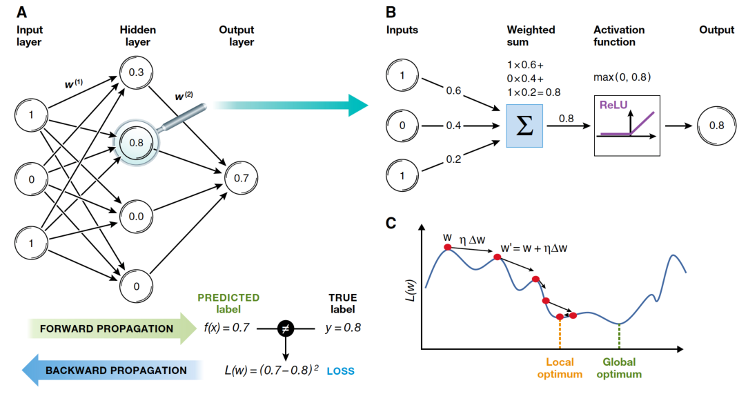
Conceptual Idea
Conceptual Idea (continued)
Conceptual Idea (continued)
Applying the chain rule recursively
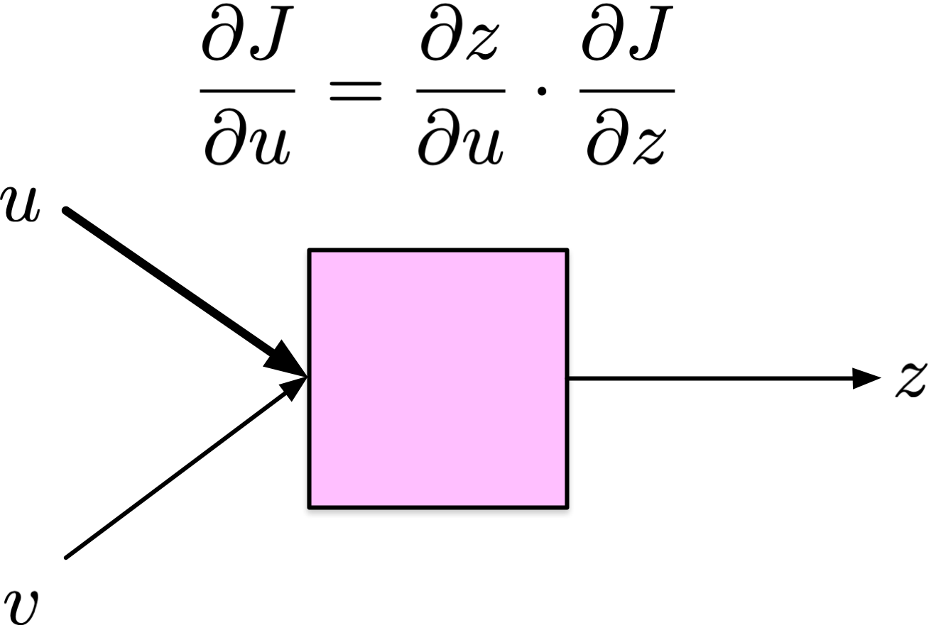
Computational graph
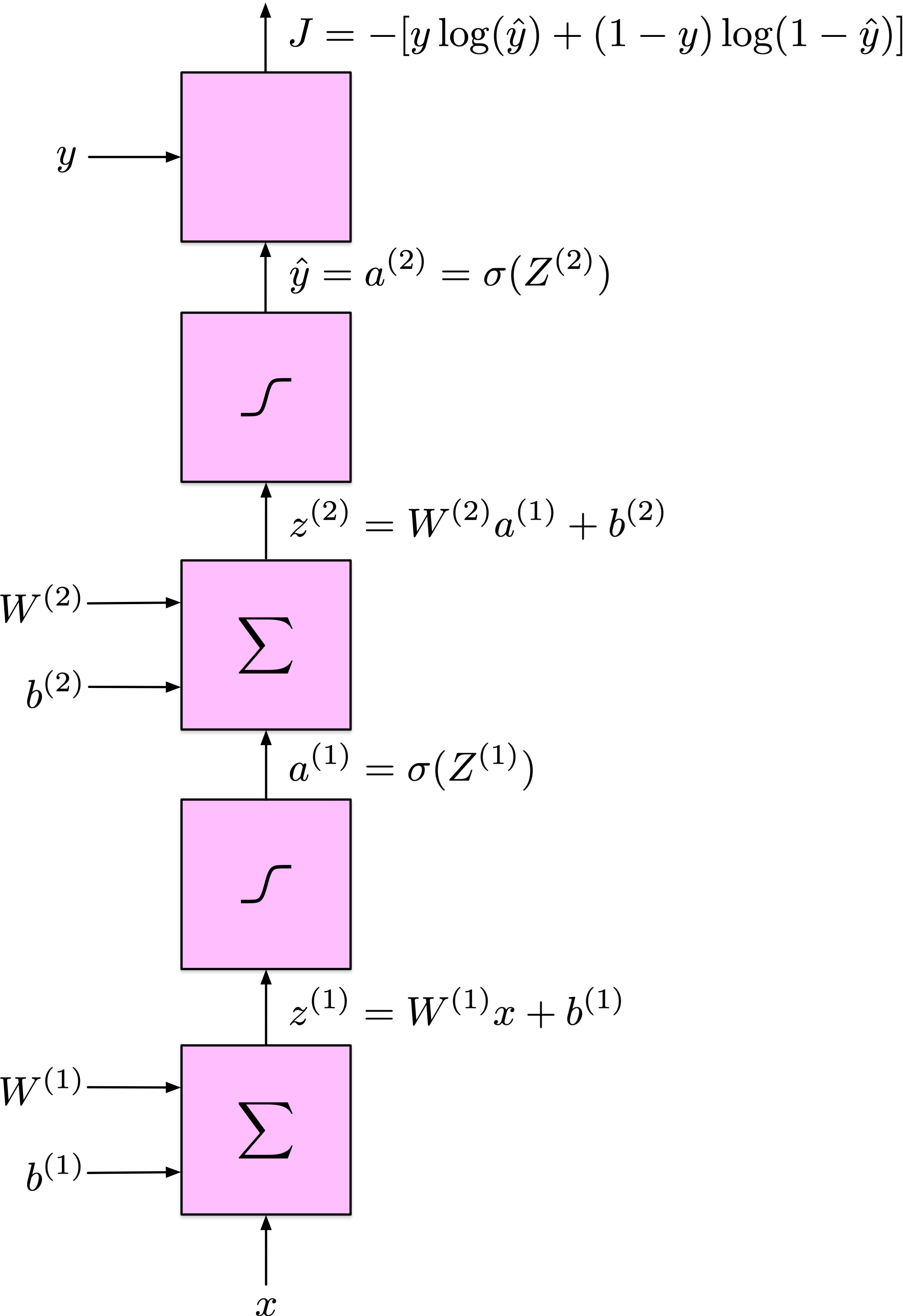
Derivatives
\[ \frac{\partial J}{\partial \hat{y}} \]
\[ \frac{\partial \hat{y}}{\partial z_2} \]
\[ \frac{\partial z_2}{\partial w_2}, \quad \frac{\partial z_2}{\partial b_2}, \quad \frac{\partial z_2}{\partial a_1}, \]
\[ \frac{\partial a_1}{\partial z_1}, \]
\[ \frac{\partial z_1}{\partial w_1}, \quad \frac{\partial z_1}{\partial b_1}, \quad \frac{\partial z_1}{\partial x}, \]
Derivatives
Loss derivative w.r.t. \(\hat{y}\):
\[ \frac{\partial J}{\partial \hat{y}} = -\left(\frac{y}{\hat{y}}-\frac{1-y}{1-\hat{y}}\right) \]
Derivatives
\(\hat{y}\) derivative w.r.t. \(z_2\):
\[ \frac{\partial \hat{y}}{\partial z_2}=\sigma^{\prime}\left(z_2\right)=\hat{y}(1-\hat{y}) \]
Derivatives
Derivative \(z_2 = w_2 a_1 + b_2\):
\[ \frac{\partial z_2}{\partial w_2}=a_1, \quad \frac{\partial z_2}{\partial b_2}=1, \quad \frac{\partial z_2}{\partial a_1}=w_2 \]
Derivatives
Derivative \(a_1 = \sigma(z_1)\):
\[ \frac{\partial a_1}{\partial z_1}=\sigma^{\prime}\left(z_1\right)=a_1\left(1-a_1\right) \]
Derivatives
Derivative \(z_1 = w_1 x + b_1\):
\[ \frac{\partial z_1}{\partial w_1}=x, \quad \frac{\partial z_1}{\partial b_1}=1, \quad \frac{\partial z_1}{\partial x} = w_1 \]
Combined derivatives
For \(w_2\):
\[ \frac{\partial J}{\partial w_2}=\frac{\partial J}{\partial \hat{y}} \cdot \frac{\partial \hat{y}}{\partial z_2} \cdot \frac{\partial z_2}{\partial w_2}=\left[-\left(\frac{y}{\hat{y}}-\frac{1-y}{1-\hat{y}}\right)\right] \cdot(\hat{y}(1-\hat{y})) \cdot a_1 \]
Simplifies to:
\[ \frac{\partial J}{\partial w_2}=(\hat{y}-y) a_1 \]
Combined derivatives
For \(b_2\):
\[ \frac{\partial J}{\partial b_2}=\frac{\partial J}{\partial \hat{y}} \cdot \frac{\partial \hat{y}}{\partial z_2} \cdot \frac{\partial z_2}{\partial b_2}=(\hat{y}-y) \cdot 1=\hat{y}-y \]
Combined derivatives
For \(w_1\):
\[ \frac{\partial J}{\partial w_1}=\frac{\partial J}{\partial \hat{y}} \cdot \frac{\partial \hat{y}}{\partial z_2} \cdot \frac{\partial z_2}{\partial a_1} \cdot \frac{\partial a_1}{\partial z_1} \cdot \frac{\partial z_1}{\partial w_1} \]
Plug in:
\[ =\left[-\left(\frac{y}{\hat{y}}-\frac{1-y}{1-\hat{y}}\right)\right] \cdot(\hat{y}(1-\hat{y})) \cdot w_2 \cdot\left(a_1\left(1-a_1\right)\right) \cdot x \]
Simplifies to:
\[ \frac{\partial J}{\partial w_1}=(\hat{y}-y) w_2\left(a_1\left(1-a_1\right)\right) x \]
Combined derivatives
For \(b_1\):
\[ \frac{\partial J}{\partial b_1}=\frac{\partial J}{\partial \hat{y}} \cdot \frac{\partial \hat{y}}{\partial z_2} \cdot \frac{\partial z_2}{\partial a_1} \cdot \frac{\partial a_1}{\partial z_1} \cdot \frac{\partial z_1}{\partial b_1} \]
Plug in:
\[ =(\hat{y}-y) w_2\left(a_1\left(1-a_1\right)\right) \cdot 1 \]
Simplifies to:
\[ \frac{\partial J}{\partial b_1}=(\hat{y}-y) w_2\left(a_1\left(1-a_1\right)\right) \]
Key derivatives
\[ \begin{align} \frac{\partial J}{\partial w_2} & = (\hat{y}-y) a_1 \\ \frac{\partial J}{\partial b_2} & = \hat{y}-y \\ \frac{\partial J}{\partial w_1} & = (\hat{y}-y) w_2\left(a_1\left(1-a_1\right)\right) x \\ \frac{\partial J}{\partial b_1} & = (\hat{y}-y) w_2\left(a_1\left(1-a_1\right)\right) \\ \end{align} \]
Key derivatives
\[ \begin{align} \frac{\partial J}{\partial w_2} & = \frac{\partial J}{\partial \hat{y}} \cdot \frac{\partial \hat{y}}{\partial z_2} \cdot \frac{\partial z_2}{\partial w_2}\\ \frac{\partial J}{\partial b_2} & = \frac{\partial J}{\partial \hat{y}} \cdot \frac{\partial \hat{y}}{\partial z_2} \cdot \frac{\partial z_2}{\partial b_2}\\ \frac{\partial J}{\partial w_1} & = \frac{\partial J}{\partial \hat{y}} \cdot \frac{\partial \hat{y}}{\partial z_2} \cdot \frac{\partial z_2}{\partial a_1} \cdot \frac{\partial a_1}{\partial z_1} \cdot \frac{\partial z_1}{\partial w_1}\\ \frac{\partial J}{\partial b_1} & = \frac{\partial J}{\partial \hat{y}} \cdot \frac{\partial \hat{y}}{\partial z_2} \cdot \frac{\partial z_2}{\partial a_1} \cdot \frac{\partial a_1}{\partial z_1} \cdot \frac{\partial z_1}{\partial b_1}\\ \end{align} \]
Key derivatives
Let \[ \begin{align} \delta_1 & = \frac{\partial J}{\partial \hat{y}} \cdot \frac{\partial \hat{y}}{\partial z_2} \\ \delta_2 & = \delta_1 \cdot \frac{\partial z_2}{\partial a_1} \cdot \frac{\partial a_1}{\partial z_1} \end{align} \]
Rewrite \[ \begin{align} \frac{\partial J}{\partial w_2} & = \delta_1 \cdot \frac{\partial z_2}{\partial w_2}\\ \frac{\partial J}{\partial b_2} & = \delta_1 \cdot \frac{\partial z_2}{\partial b_2}\\ \frac{\partial J}{\partial w_1} & = \delta_2 \cdot \frac{\partial z_1}{\partial w_1}\\ \frac{\partial J}{\partial b_1} & = \delta_2 \cdot \frac{\partial z_1}{\partial b_1}\\ \end{align} \]
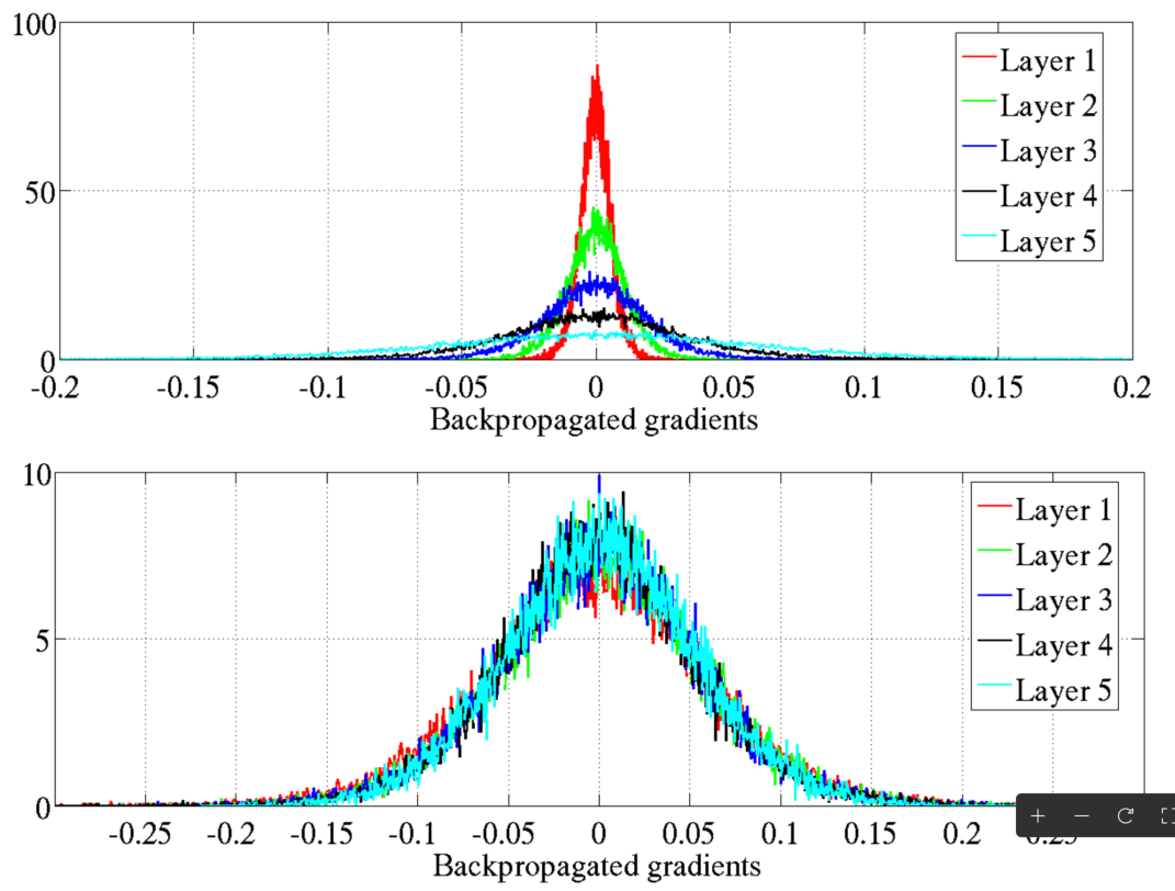
Glorot and Bengio
Figure 6
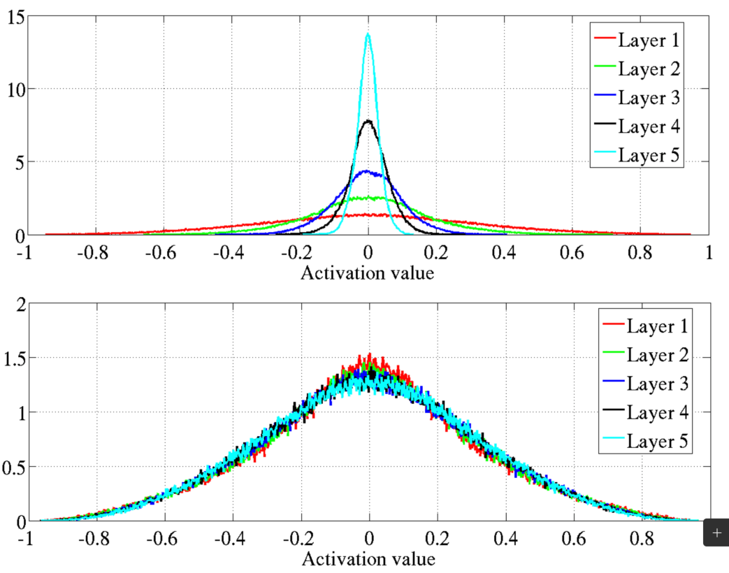
Figure 7
Activation Function: Leaky ReLU
Show code
import numpy as np
import matplotlib.pyplot as plt

# Define the Leaky ReLU function
def leaky_relu(x, alpha=0.21):
    return np.where(x > 0, x, alpha * x)

# Define the derivative of the Leaky ReLU function
def leaky_relu_derivative(x, alpha=0.2):
    return np.where(x > 0, 1, alpha)

# Generate a range of input values
x_values = np.linspace(-4, 4, 400)

# Compute the Leaky ReLU and its derivative
leaky_relu_values = leaky_relu(x_values)
leaky_relu_derivative_values = leaky_relu_derivative(x_values)

# Create the plot
plt.figure(figsize=(5, 3))

# Plot the Leaky ReLU
plt.subplot(1, 2, 1)
plt.plot(x_values, leaky_relu_values, label='Leaky ReLU', color='blue')
plt.title('Leaky ReLU Activation Function')
plt.xlabel('x')
plt.ylabel('f(x)')
plt.grid(True)
plt.axhline(0, color='black',linewidth=0.5)
plt.axvline(0, color='black',linewidth=0.5)
plt.legend()

# Plot the derivative of the Leaky ReLU
plt.subplot(1, 2, 2)
plt.plot(x_values, leaky_relu_derivative_values, label='Derivative of Leaky ReLU', color='red')
plt.title('Derivative of Leaky ReLU')
plt.xlabel('x')
plt.ylabel("f'(x)")
plt.grid(True)
plt.axhline(0, color='black',linewidth=0.5)
plt.axvline(0, color='black',linewidth=0.5)
plt.legend()

# Show the plots
plt.tight_layout()
plt.show()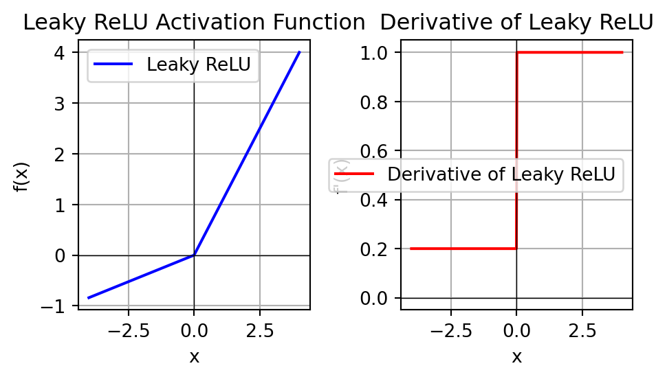
Summary