Introduction to Search

CSI 4106

Marcel Turcotte

Version: Nov 7, 2025 09:01

Preamble

Message of the Day

Learning Objectives

  • Describe the role of search algorithms in AI, crucial for planning, reasoning, and applications like AlphaGo.
  • Recall key search concepts: state space, initial/goal states, actions, transition models, cost functions.
  • Identify the differences of uninformed search algorithms (BFS and DFS).
  • Implement BFS and DFS and compare them using the 8-Puzzle problem.
  • Analyze performance and optimality of various search algorithms.

Justification

Justification

Justification

We have honed our expertise in machine learning to a point where we possess a robust understanding of neural networks and deep learning, allowing us to develop simple models using Keras.

In recent years, Monte Carlo Tree Search (MCTS) has played a pivotal role in advancing artificial intelligence research. After initially concentrating on deep learning, we are now shifting our focus to search.

Justification

The integration of deep learning and MCTS underpins modern applications such as AlphaGo, AlphaZero, and MuZero.

Search algorithms are crucial in addressing challenges in planning and reasoning and are likely to become increasingly significant in future developments.

Search (a biased timeline)

  • 1968 – A*: Heuristic-based search, foundational for pathfinding and planning in AI.
  • 1970s-1980s – Population-Based Algorithms (e.g., Genetic Algorithms): Stochastic optimization approaches useful for large, complex search spaces.
  • 1980s – Constraint Satisfaction Problems (CSPs): Search in structured spaces with explicit constraints; a precursor to formal problem-solving systems.
  • 2013 – DQN: Reinforcement learning via search (Q-learning) from raw input (pixels).
  • 2015 – AlphaGo: Game-tree search with Monte Carlo Tree Search (MCTS) combined with deep learning.
  • 2017 – AlphaZero: Generalized self-play with MCTS in multiple domains.
  • 2019 – MuZero: Search in unknown environments without predefined models.
  • 2020 – Agent57: Generalized search across multiple environments (Atari games).
  • 2020 – AlphaGeometry: Search-based theorem proving in mathematical spaces.
  • 2021 – FunSearch: Potentially another generalization of search techniques.

AlphaGo - The Movie

AlphaGo2MuZero

Search

Applications

  • Pathfinding and Navigation: Used in robotics and video games to find a path from a starting point to a destination.
  • Puzzle Solving: Solving puzzles like the 8-puzzle, mazes, or Sudoku.
  • Network Analysis: Analyzing networks and graphs, such as finding connectivity or shortest paths in social networks or transportation maps.
  • Game Playing: Used to evaluate moves in games like chess or Go, especially when combined with other strategies.

Applications

  • Scheduling: Planning and scheduling tasks in manufacturing, project management, or airline scheduling.
  • Resource Allocation: Allocating resources in a network or within an organization where constraints must be satisfied.
  • Configuration Problems: Solving problems where a set of components must be assembled to meet specific requirements, such as configuring a computer system or designing a circuit.

Applications

  • Decision Making under Uncertainty: Used in real-time strategy games and simulations where decisions need to be evaluated under uncertain conditions.

  • Storrytelling: LLMs can effectively generate stories when guided by a valid input plan from an automated planner. (Simon and Muise 2024)

Outline

  1. Deterministic & Heuristic Search: BFS, DFS, A* for pathfinding and optimization in classical AI.

  2. Population-Based Algorithms: Focus on structured problems and stochastic search.

  3. Adversarial Game Algorithms: Minimax, alpha-beta pruning, MCTS for decision-making in competitive environments.

Definition

When the correct action to take is not immediately obvious, an agent may need to to plan ahead: to consider a sequence of actions that form a path to a goal state. Such an agent is called a problem-solving agent, and the computational process it undertakes is called search.

Terminology

Environment Characteristics

  • Observability: Partially observable, or fully observable
  • Agent Composition: Single or multiple agents
  • Predictability: Deterministic or non-deterministic
  • State Dependency: Stateless or stateful
  • Temporal Dynamics: Static or dynamic
  • State Representation: Discrete or continuous

Problem-Solving Process

Search: The process involves simulating sequences of actions until the agent achieves its goal. A successful sequence is termed a solution.

Search Problem Definition

  • A collection of states, referred to as the state space.

  • An initial state where the agent begins.

  • One or more goal states that define successful outcomes.

  • A set of actions available in a given state \(s\).

  • A transition model that determines the next state based on the current state and selected action.

  • An action cost function that specifies the cost of performing action \(a\) in state \(s\) to reach state \(s'\).

Definitions

  • A path is defined as a sequence of actions.
  • A solution is a path that connects the initial state to the goal state.
  • An optimal solution is the path with the lowest cost among all possible solutions.

Example: 8-Puzzle

Code
import random
import matplotlib.pyplot as plt
import numpy as np

random.seed(58)

def is_solvable(tiles):
    # Count the inversions in the flattened list of tiles (excluding the blank space).
    # Assumption: board is square and width is odd.
    inversions = 0
    for i in range(len(tiles)):
        for j in range(i + 1, len(tiles)):
            if tiles[i] != 0 and tiles[j] != 0 and tiles[i] > tiles[j]:
                inversions += 1
    return inversions % 2 == 0

def generate_solvable_board():
    # Generate a random board configuration that is guaranteed to be solvable
    tiles = list(range(9))
    random.shuffle(tiles)
    while not is_solvable(tiles):
        random.shuffle(tiles)

    return tiles

def plot_board(board, title, num_pos, position):
    ax = plt.subplot(1, num_pos, position)
    ax.set_title(title)
    ax.set_xticks([])
    ax.set_yticks([])

    board = np.array(board).reshape(3, 3).tolist() # Reconfigure the grid to be 3x3

    # Use a color map to display the numbers
    cmap = plt.cm.plasma
    norm = plt.Normalize(vmin=-1, vmax=8)

    for i in range(3):
        for j in range(3):
            tile_value = board[i][j]
            color = cmap(norm(tile_value))
            ax.add_patch(plt.Rectangle((j, 2 - i), 1, 1, facecolor=color, edgecolor='black'))
            if tile_value == 0:
                ax.add_patch(plt.Rectangle((j, 2 - i), 1, 1, facecolor='white', edgecolor='black'))
            else:
                ax.text(j + 0.5, 2 - i + 0.5, str(tile_value),
                        fontsize=16, ha='center', va='center', color='black')

    ax.set_xlim(0, 3)
    ax.set_ylim(0, 3)

Example: 8-Puzzle

Code
# Generate initial solvable board
initial_board = generate_solvable_board()

# Define goal state
goal_board = [
    [1, 2, 3],
    [4, 5, 6],
    [7, 8, 0]
]

# Plot both boards
plt.figure(figsize=(8, 4))
plot_board(initial_board, "Initial Board", 2, 1)
plot_board(goal_board, "Goal State", 2, 2)
plt.tight_layout()
plt.show()

8-Puzzle

  • How can the states be represented?

  • What constitutes the initial state?

  • What defines the actions?

  • What would constitute a path?

  • What characterizes the goal state?

  • What would constitute a solution?

  • What should be the cost of an action?

Are all the boards solvable?

Are all the boards solvable?

  • A board is solvable if it has the same inversion parity as the goal state.

  • An inversion is a pair of tiles (excluding the blank) that are in the wrong order relative to each other, when reading the board as a one-dimensional list (left-to-right, top-to-bottom).

  • When the goal is the ordered sequence from 1 to 8, there are no inversion, and therefore parity is even.

  • See Archer (1999) or Slider Puzzle, Princeton

count_even_odd_parity

Code
from itertools import permutations

def count_even_odd_parity():
    even_count = 0
    odd_count = 0

    for perm in permutations(range(9)):  # 0 represents the blank
        inversions = 0
        for i in range(9):
            for j in range(i + 1, 9):
                if perm[i] != 0 and perm[j] != 0 and perm[i] > perm[j]:
                    inversions += 1
        if inversions % 2 == 0:
            even_count += 1
        else:
            odd_count += 1

    return even_count, odd_count
even, odd = count_even_odd_parity()

print(f"Even parity: {even}")
print(f"Odd parity: {odd}")
Even parity: 181440
Odd parity: 181440

Search Tree

Search Tree

Search Tree

  • The root of the search tree represents the initial state of the problem.

  • Expanding a node involves evaluating all possible actions available from that state.

  • The result of an action is the new state achieved after applying that action to the current state.

  • Similar to other tree structures, each node (except for the root and leaf nodes) has a parent and may have children.

Frontier

Frontier

Frontier

Definition

An uninformed search (or blind search) is a search strategy that explores the search space using only the information available in the problem definition, without any domain-specific knowledge, evaluating nodes based solely on their inherent properties rather than estimated costs or heuristics.

State Representation

Code
# Plot both boards
initial_state_8 = [6, 4, 5,
                    8, 2, 7,
                    1, 0, 3]
goal_state_8 = [1, 2, 3,
                4, 5, 6,
                7, 8, 0]

plt.figure(figsize=(4, 2))
plot_board(initial_state_8, "Initial Board", 2, 1)
plot_board(goal_state_8, "Goal State", 2, 2)
plt.tight_layout()
plt.show()

initial_state_8 = [6, 4, 5,
                   8, 2, 7,
                   1, 0, 3]

goal_state_8 = [1, 2, 3,
                4, 5, 6,
                7, 8, 0]

is_goal

def is_goal(state, goal_state):
    """Determines if a given state matches the goal state."""
    return state == goal_state

expand

def expand(state):
    """Generates successor states by moving the blank tile in all possible directions."""
    size = int(len(state) ** 0.5)  # Determine puzzle size (3 for 8-puzzle, 4 for 15-puzzle)
    idx = state.index(0)  # Find the index of the blank tile represented by 0
    x, y = idx % size, idx // size  # Convert index to (x, y) coordinates
    neighbors = []

    # Define possible moves: Left, Right, Up, Down
    moves = [(-1, 0), (1, 0), (0, -1), (0, 1)]
    for dx, dy in moves:
        nx, ny = x + dx, y + dy
        # Check if the new position is within the puzzle boundaries
        if 0 <= nx < size and 0 <= ny < size:
            n_idx = ny * size + nx
            new_state = state.copy()
            # Swap the blank tile with the adjacent tile
            new_state[idx], new_state[n_idx] = new_state[n_idx], new_state[idx]
            neighbors.append(new_state)
    return neighbors

expand

Code
plt.figure(figsize=(8, 2))

solutions = expand(initial_state_8)

plot_board(initial_state_8, "Initial State", 4, 1)

for i, solution in enumerate(solutions):
    plot_board(solution, f"State: {i}", 4, i+2)

plt.tight_layout()
plt.show()

expand(initial_state_8)
[[6, 4, 5, 8, 2, 7, 0, 1, 3],
 [6, 4, 5, 8, 2, 7, 1, 3, 0],
 [6, 4, 5, 8, 0, 7, 1, 2, 3]]

is_empty

def is_empty(frontier):
    """Checks if the frontier is empty."""
    return len(frontier) == 0

Cycles

A path that revisits the same states forms a cycle.

Allowing cycles would render the resulting search tree infinite.

To prevent this, we monitor the states that have been reached, though this incurs a memory cost.

Breadth-first search

from collections import deque

Breadth-first search (BFS) employs a queue to manage the frontier nodes, which are also known as the open list.

Breadth-first search

def bfs(initial_state, goal_state):

    frontier = deque()  # Initialize the queue for BFS
    frontier.append((initial_state, []))  # Each element is a tuple: (state, path)

    explored = set()
    explored.add(tuple(initial_state))

    iterations = 0 # simply used to compare algorithms

    while not is_empty(frontier):
        current_state, path = frontier.popleft()

        if is_goal(current_state, goal_state):
            print(f"Number of iterations: {iterations}")
            return path + [current_state]  # Return the successful path

        iterations = iterations + 1

        for neighbor in expand(current_state):
            neighbor_tuple = tuple(neighbor)
            if neighbor_tuple not in explored:
                explored.add(neighbor_tuple)
                frontier.append((neighbor, path + [current_state]))

    return None  # No solution found

Simple Case

Code
plt.figure(figsize=(8, 2))

initial_state_8 = [1, 2, 3,
                   4, 0, 6,
                   7, 5, 8]
goal_state_8 = [1, 2, 3,
                4, 5, 6,
                7, 8, 0]

solutions = bfs(initial_state_8, goal_state_8)

for i, solution in enumerate(solutions):
    plot_board(solution, f"Step: {i}", 3, i+1)

plt.tight_layout()
plt.show()
Number of iterations: 12

initial_state_8 = [1, 2, 3,
                   4, 0, 6,
                   7, 5, 8]
goal_state_8 = [1, 2, 3,
                4, 5, 6,
                7, 8, 0]

bfs(initial_state_8, goal_state_8)
Number of iterations: 12
[[1, 2, 3, 4, 0, 6, 7, 5, 8],
 [1, 2, 3, 4, 5, 6, 7, 0, 8],
 [1, 2, 3, 4, 5, 6, 7, 8, 0]]

Challenging Case

initial_state_8 = [6, 4, 5,
                   8, 2, 7,
                   1, 0, 3]
goal_state_8 = [1, 2, 3,
                4, 5, 6,
                7, 8, 0]

print("Solving 8-puzzle with BFS...")

solution_8_bfs = bfs(initial_state_8, goal_state_8)

if solution_8_bfs:
    print(f"BFS Solution found in {len(solution_8_bfs) - 1} moves:")
    print_solution(solution_8_bfs)
else:
    print("No solution found for 8-puzzle using BFS.")
Solving 8-puzzle with BFS...
Number of iterations: 145605
BFS Solution found in 25 moves:
Step 0:
6 4 5
8 2 7
1   3

Step 1:
6 4 5
8 2 7
  1 3

Step 2:
6 4 5
  2 7
8 1 3

Step 3:
6 4 5
2   7
8 1 3

Step 4:
6   5
2 4 7
8 1 3

Step 5:
  6 5
2 4 7
8 1 3

Step 6:
2 6 5
  4 7
8 1 3

Step 7:
2 6 5
4   7
8 1 3

Step 8:
2 6 5
4 1 7
8   3

Step 9:
2 6 5
4 1 7
  8 3

Step 10:
2 6 5
  1 7
4 8 3

Step 11:
2 6 5
1   7
4 8 3

Step 12:
2 6 5
1 7  
4 8 3

Step 13:
2 6 5
1 7 3
4 8  

Step 14:
2 6 5
1 7 3
4   8

Step 15:
2 6 5
1   3
4 7 8

Step 16:
2   5
1 6 3
4 7 8

Step 17:
2 5  
1 6 3
4 7 8

Step 18:
2 5 3
1 6  
4 7 8

Step 19:
2 5 3
1   6
4 7 8

Step 20:
2   3
1 5 6
4 7 8

Step 21:
  2 3
1 5 6
4 7 8

Step 22:
1 2 3
  5 6
4 7 8

Step 23:
1 2 3
4 5 6
  7 8

Step 24:
1 2 3
4 5 6
7   8

Step 25:
1 2 3
4 5 6
7 8  

BFS Search Tree

Depth-First Search

def dfs(initial_state, goal_state):

    frontier = [(initial_state, [])]  # Each element is a tuple: (state, path)

    explored = set()
    explored.add(tuple(initial_state))

    iterations = 0

    while not is_empty(frontier):
        current_state, path = frontier.pop()

        if is_goal(current_state, goal_state):
            print(f"Number of iterations: {iterations}")
            return path + [current_state]  # Return the successful path

        iterations = iterations + 1

        for neighbor in expand(current_state):
            neighbor_tuple = tuple(neighbor)
            if neighbor_tuple not in explored:
                explored.add(neighbor_tuple)
                frontier.append((neighbor, path + [current_state]))

    return None  # No solution found

DFS Search Tree

DFS Search Tree

Simple Case

Code
plt.figure(figsize=(8, 2))

initial_state_8 = [1, 2, 3,
                   4, 0, 6,
                   7, 5, 8]
goal_state_8 = [1, 2, 3,
                4, 5, 6,
                7, 8, 0]

solutions = dfs(initial_state_8, goal_state_8)

for i, solution in enumerate(solutions):
    plot_board(solution, f"Step: {i}", 3, i+1)

plt.tight_layout()
plt.show()
Number of iterations: 2

initial_state_8 = [1, 2, 3,
                   4, 0, 6,
                   7, 5, 8]
goal_state_8 = [1, 2, 3,
                4, 5, 6,
                7, 8, 0]

bfs(initial_state_8, goal_state_8)
Number of iterations: 12
[[1, 2, 3, 4, 0, 6, 7, 5, 8],
 [1, 2, 3, 4, 5, 6, 7, 0, 8],
 [1, 2, 3, 4, 5, 6, 7, 8, 0]]

Challenging Case

initial_state_8 = [6, 4, 5,
                   8, 2, 7,
                   1, 0, 3]
goal_state_8 = [1, 2, 3,
                4, 5, 6,
                7, 8, 0]

print("Solving 8-puzzle with DFS...")

solution_8_bfs = dfs(initial_state_8, goal_state_8)

if solution_8_bfs:
    print(f"DFS Solution found in {len(solution_8_bfs) - 1} moves:")
    # print_solution(solution_8_bfs)
else:
    print("No solution found for 8-puzzle using DFS.")
Solving 8-puzzle with DFS...
Number of iterations: 1187
DFS Solution found in 1157 moves:

Remarks

  • Breadth-first search (BFS) identifies the optimal solution, 25 moves, in 145,605 iterations.

  • Depth-first search (DFS) discovers a solution involving 1,157 moves in 1,187 iterations.

Prologue

Summary

  • Justification for Studying Search
  • Key Terminology and Concepts
  • Uninformed Search Algorithms
    • Breadth-First Search (BFS)
    • Depth-First Search (DFS)
  • Implementations

Next lecture

  • We will further explore heuristic functions and examine additional search algorithms.

References

Archer, Aaron F. 1999. “A Modern Treatment of the 15 Puzzle.” The American Mathematical Monthly 106 (9): 793–99. https://doi.org/10.1080/00029890.1999.12005124.
Russell, Stuart, and Peter Norvig. 2020. Artificial Intelligence: A Modern Approach. 4th ed. Pearson. http://aima.cs.berkeley.edu/.
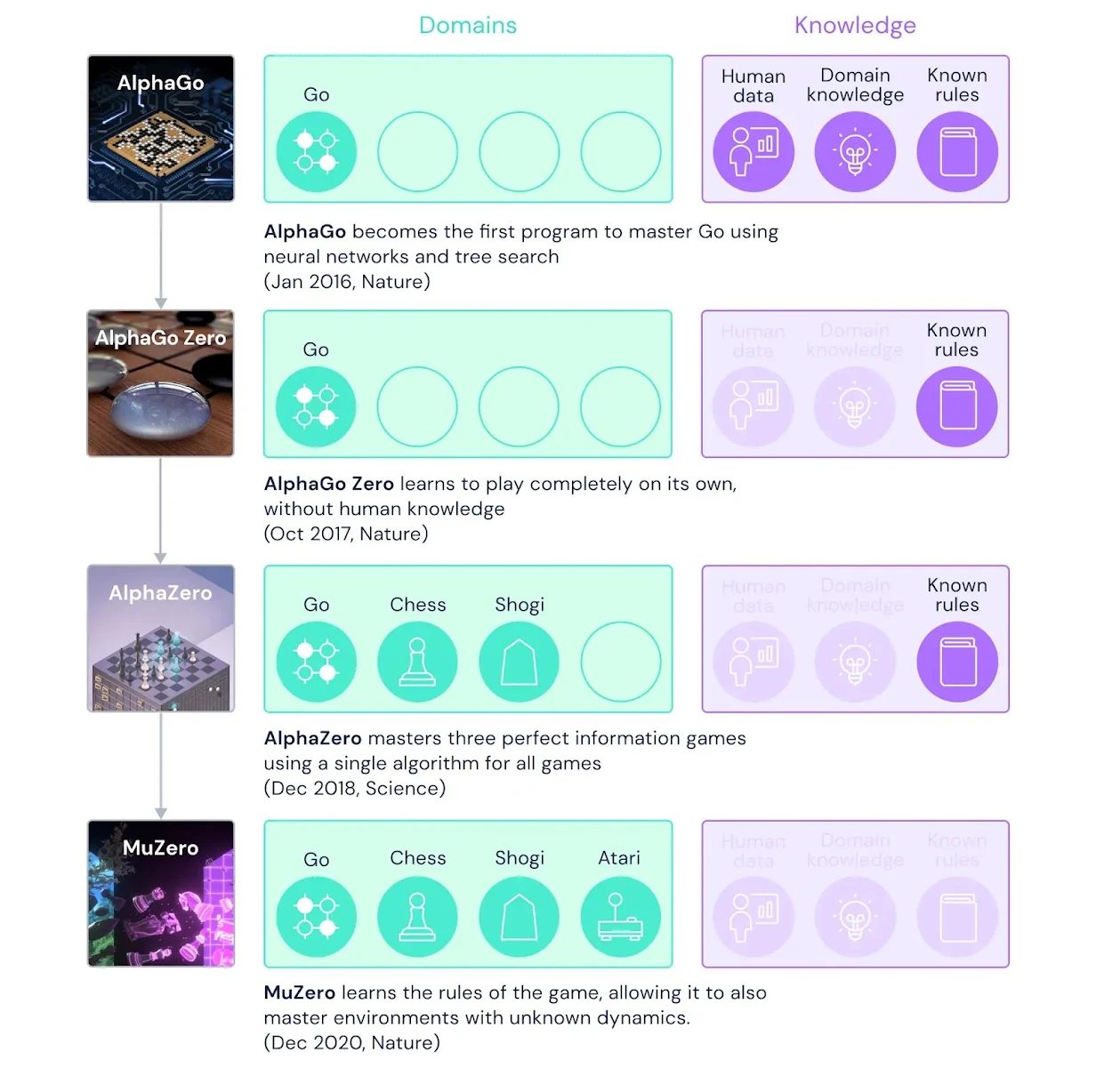
Schrittwieser, Julian, Ioannis Antonoglou, Thomas Hubert, Karen Simonyan, Laurent Sifre, Simon Schmitt, Arthur Guez, et al. 2020. Mastering Atari, Go, chess and shogi by planning with a learned model.” Nature 588 (7839): 604–9. https://doi.org/10.1038/s41586-020-03051-4.
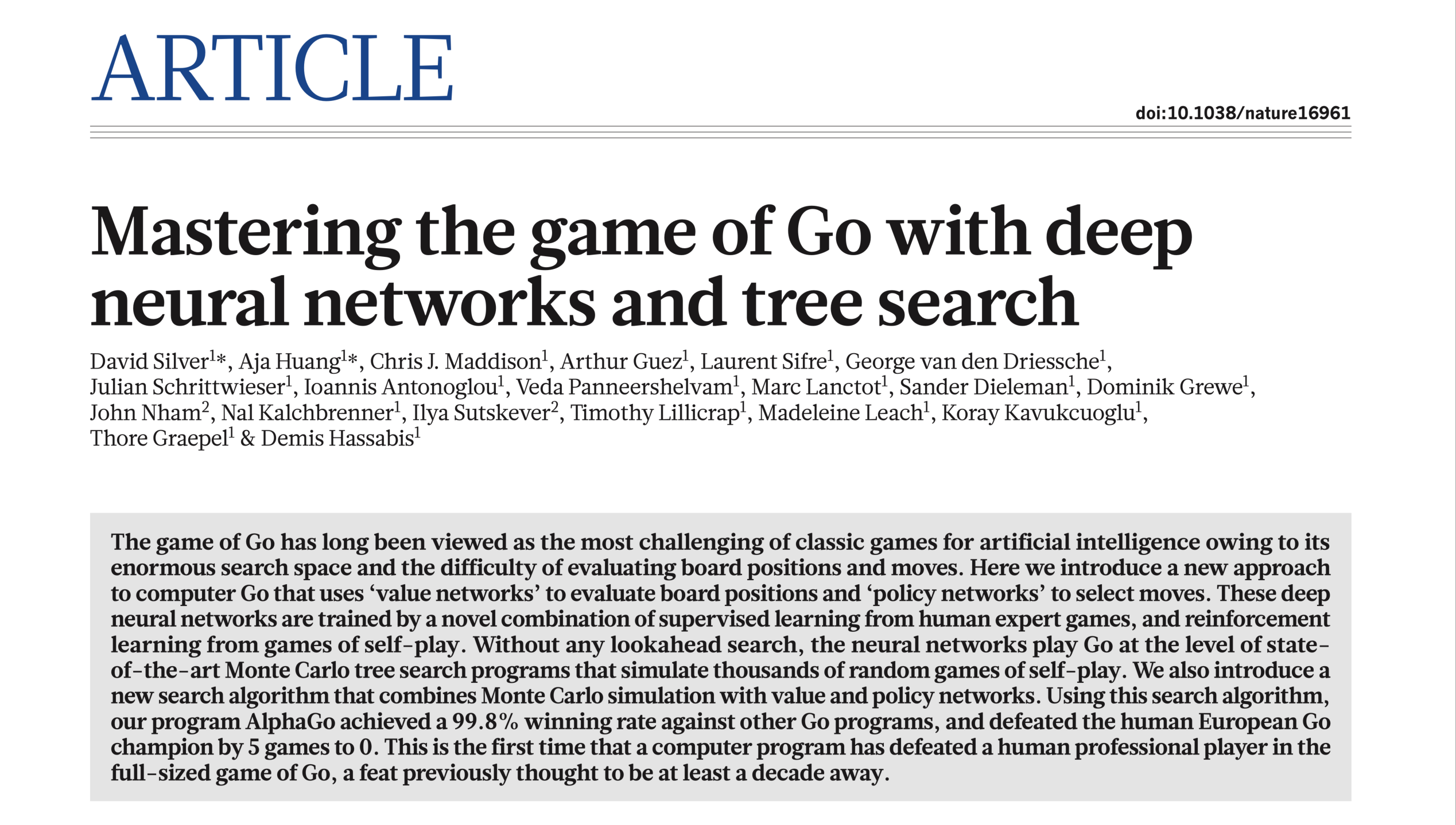
Silver, David, Aja Huang, Chris J. Maddison, Arthur Guez, Laurent Sifre, George van den Driessche, Julian Schrittwieser, et al. 2016. Mastering the game of Go with deep neural networks and tree search.” Nature 529 (7587): 484–89. https://doi.org/10.1038/nature16961.
Simon, Nisha, and Christian Muise. 2024. “Want To Choose Your Own Adventure? Then First Make a Plan.” Proceedings of the Canadian Conference on Artificial Intelligence.

Marcel Turcotte

Marcel.Turcotte@uOttawa.ca

School of Electrical Engineering and Computer Science (EECS)

University of Ottawa