Local Search

CSI 4106 Introduction to Artificial Intelligence

Marcel Turcotte

Version: Nov 10, 2025 08:56

Preamble

Message of the Day

Universities are embracing AI: will students get smarter or stop thinking?, Nature News, 2025-10-21.

Learning Objectives

• Understand the concept and application of local search algorithms in optimization problems.
• Implement and analyze the hill-climbing algorithm, recognizing its limitations such as local maxima and plateaus.
• Apply effective state representation strategies in problems like the 8-Queens to enhance search efficiency.
• Explain how simulated annealing overcomes local optima by allowing probabilistic acceptance of worse states.
• Analyze the influence of temperature and energy difference on the acceptance probability in simulated annealing.
• Recognize the application of simulated annealing in solving complex optimization problems like the Travelling Salesman Problem (TSP).

In this presentation, we will analyze two local search algorithms: hill climbing and simulated annealing. Our goal is to explain the concept of local search and examine methods for avoiding local optima. We will briefly discuss hill climbing, given its simplicity, and spend more time on simulated annealing, a very useful algorithm.

Introduction

Context

• Focus has been on finding paths in state space.

• Some problems prioritize the goal state over the path.

  • Integrated-circuit design
  • Job shop scheduling
  • Automatic programming

The importance of the path versus the goal state hinges on the problem’s nature. For instance, in a routing problem, the path is the critical piece of information sought.

8-Queens Problem

import matplotlib.pyplot as plt
from matplotlib.colors import ListedColormap
import numpy as np

def display_n_queens(board, width):
    n = len(board)

    # Create a checkerboard pattern
    board_matrix = np.zeros((n, n))
    for row in range(n):
        for col in range(n):
            if (row + col) % 2 == 0:
                board_matrix[row, col] = 1  # White tiles
            else:
                board_matrix[row, col] = 0.5

    # Create custom colormap: gray for 0.5 and white for 1
    cmap = ListedColormap(['lightgray', 'white'])

    # Create the plot
    fig, ax = plt.subplots(figsize=(width, width))
    ax.imshow(board_matrix, cmap=cmap, extent=(0, n, 0, n))

    # Add the queen markers
    for col in range(n):
        row = board[col]
        ax.text(col + 0.5, n - row - 0.5, '♛', fontsize=32, ha='center', va='center', color='black')

    # Add grid lines
    ax.set_xticks(np.arange(n+1), minor=True)
    ax.set_yticks(np.arange(n+1), minor=True)
    ax.grid(which='minor', color='black', linestyle='-', linewidth=2)

    # Remove axis labels and ticks
    ax.set_xticks([])
    ax.set_yticks([])
    ax.tick_params(axis='both', which='both', length=0)  # Ensure ticks are completely disabled

    plt.title(f"{n}-Queens Problem")
    plt.show()

8-Queens Problem

# Example board for the 8-queens problem
# Represents one valid solution
board = [0, 4, 7, 5, 2, 6, 1, 3]  

display_n_queens(board, 5)

For an \(8 \times 8\) chessboard, there exist precisely 92 distinct solutions. Eliminating symmetry, one finds 12 fondamental solutions. In the more general scenario of an \(n \times n\) chessboard, the exact number of solutions has been determined for all \(n\) values up to and including 27.

The 8-Queens problem involves placing eight queens on an \(8 \times 8\) chessboard such that no two queens threaten each other, meaning no two queens share the same row, column, or diagonal.

Definition

(Russell and Norvig 2020, 110)

Local search algorithms operate by searching from a start state to neighboring states, without keeping track of the paths, nor the set of states that have been reached.

This algorithm lacks a systematic approach and does not ensure the discovery of an optimal solution.

Optimizes memory utilization while effectively solving problems in extensive or infinite state spaces.

Problem Definition

Find the “best” state according to an objective function, thereby locating the global maximum.

This optimization problem is commonly referred to as hill climbing.

Hill-Climbing

Hill-Climbing

Hill-Climbing

Given as in input a problem

• current is the initial state of problem

• while not done do

  • nighbour is the highest-valued successor state of current
  • if value(neighbour) \(\le\) value(current) the return current
  • set current to neighbour

Hill climbing neither records previously visited states nor anticipates beyond its immediate neighbors. It keeps track of one current state moves in the direction of the steepest ascent.

Notably, by inverting the sign of the objective function, the algorithm can be adapted to seek a local minimum instead.

8-Queens

How would you represent the current state?

Why is using a grid to represent the current state suboptimal?

A grid representation permits the illegal placement of two queens in the same column.

Instead, we can represent the state as a list (\(\mathrm{state}\)), where each element corresponds to the row position of the queen in its respective column.

In other words, \(\mathrm{state}[i]\) is the row of the queen is column \(i\).

State Representation

# Example board for the 8-queens problem
board = [0, 4, 7, 5, 2, 6, 1, 3]  # Represents one valid solution for 8-queens

display_n_queens(board, 5)

state = [0, 4, 7, 5, 2, 6, 1, 3]

create_initial_state

import random
random.seed(7)

def create_initial_state(n):

    """Generates a random initial state with one queen per column."""

    return [random.randint(0, n - 1) for _ in range(n)]

What do you think?

create_initial_state

state = create_initial_state(8)
display_n_queens(state, 5)

state 

[5, 2, 6, 0, 1, 1, 5, 0]

Permits two queens in the same row? How can this be resolved?

Representation of 8-Queens

\(8 \times 8\) chessboard.

• Unconstrained Placement: \(\binom{64}{8} = 4,426,165,368\) possible configurations, representing the selection of 8 squares from 64.

• Column Constraint: Use a list of length 8, with each entry indicating the row of a queen in its respective column, resulting in \(8^8 = 16,777,216\) configurations.

• Row and Column Constraints: Model board states as permutations of the 8 row indices, reducing configurations to \(8! = 40,320\).

This underscores the significance of selecting a good representation.

create_initial_state

import random
random.seed(7)

def create_initial_state(n):

    """Generates a permutation of numbers from 0 to n-1 as the initial state."""

    state = list(range(n))
    random.shuffle(state)

    return state

create_initial_state

state = create_initial_state(8)
display_n_queens(state, 5)

state 

[6, 7, 2, 4, 0, 3, 1, 5]

calculate_conflicts

def calculate_conflicts(state):

    n = len(state)
    conflicts = 0

    for col_i in range(n):
        for col_j in range(col_i + 1, n):
            row_i = state[col_i]
            row_j = state[col_j]
            if row_i == row_j:                 # same row
                conflicts += 1
            if col_i - row_i == col_j - row_j: # same diagonal
                conflicts += 1
            if col_i + row_i == col_j + row_j: # same anti-diagonal
                conflicts += 1

    return conflicts

calculate_conflicts

display_n_queens(state, 5)

5

get_neighbors_rn

def get_neighbors_rn(state):

    """Generates neighboring states by moving on queen at a time to a new row."""

    neighbors = []
    n = len(state)

    for col in range(n):
        for row in range(n):
            if (state[col] != row):
              new_state = state[:] # create a copy of the state
              new_state[col] = row
              neighbors.append(new_state)

    return neighbors

Russell and Norvig (2020), \(8 \times 7 = 56\) neighbours

get_neighbors_rn

etat = create_initial_state(8)
display_n_queens(etat, 5)

get_neighbors_rn

initial_state_8 = create_initial_state(8)
print(initial_state_8)
for s in get_neighbors_rn(initial_state_8):
  print(f"{s} -> # of conflicts = {calculate_conflicts(s)}")

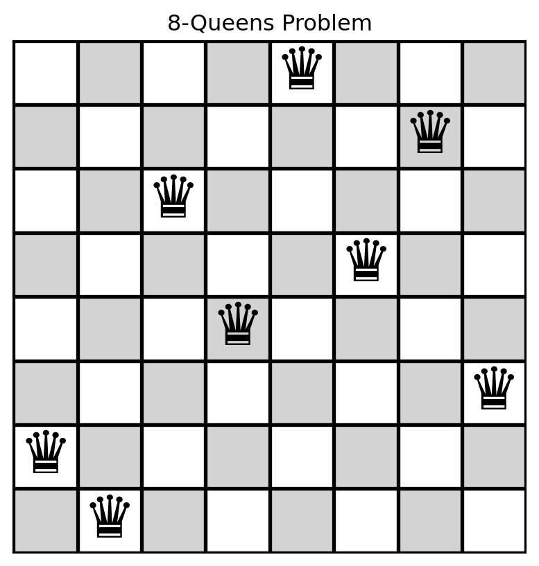
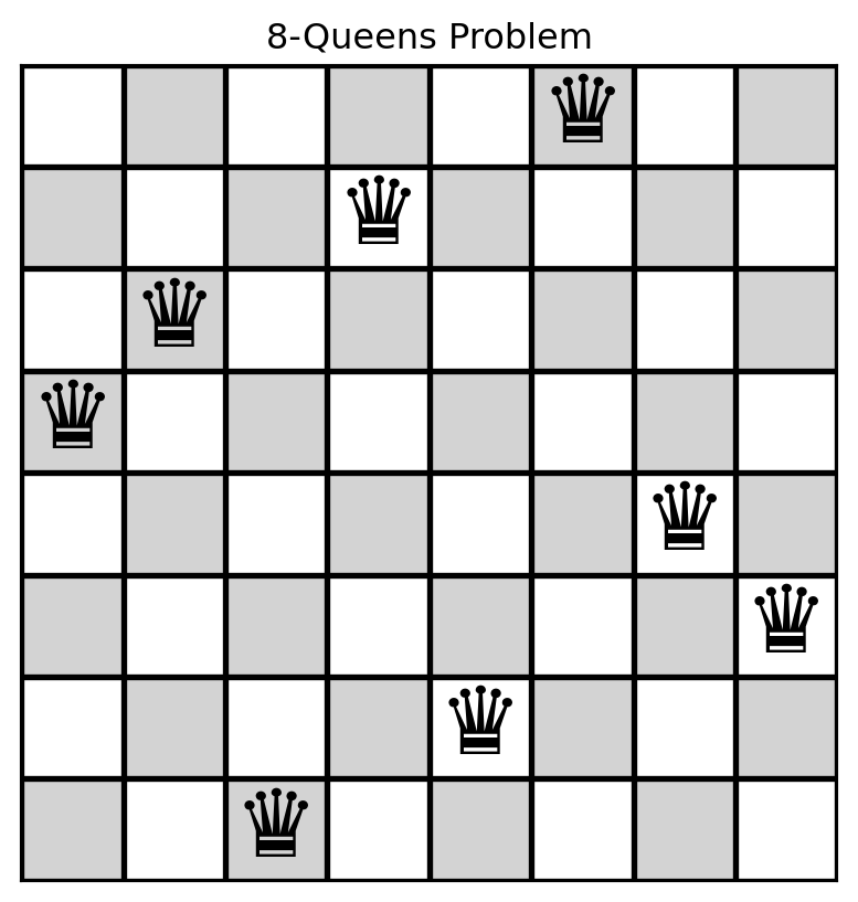
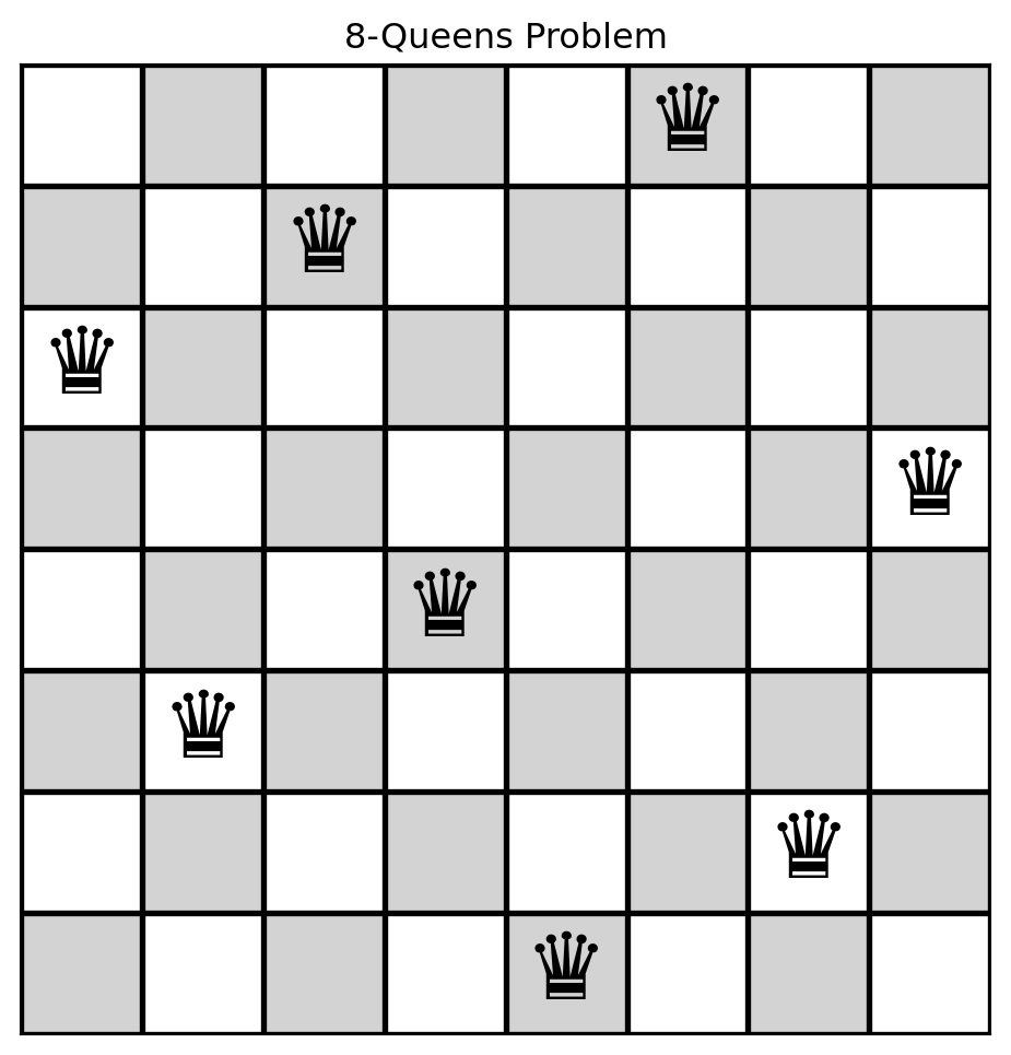
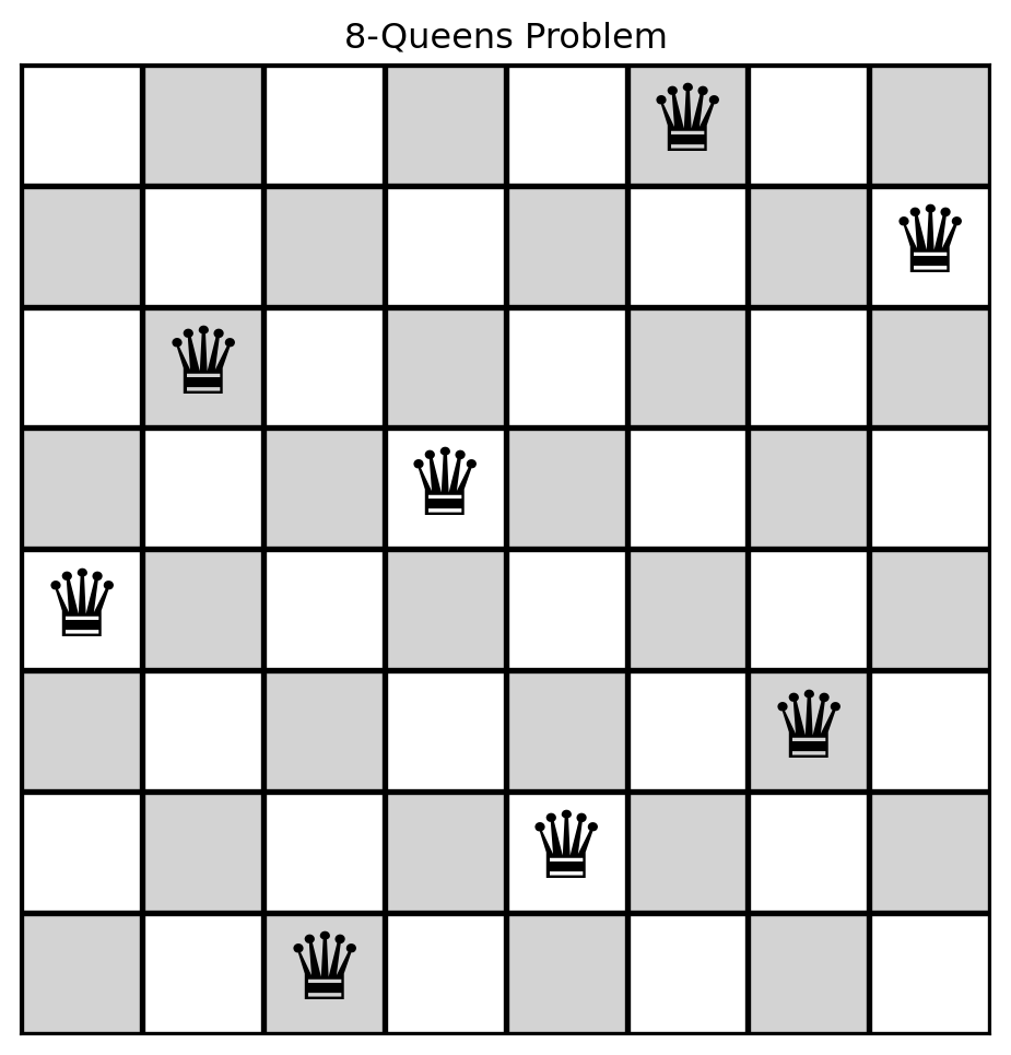
[7, 4, 2, 5, 1, 0, 3, 6]
[0, 4, 2, 5, 1, 0, 3, 6] -> # of conflicts = 6
[1, 4, 2, 5, 1, 0, 3, 6] -> # of conflicts = 5
[2, 4, 2, 5, 1, 0, 3, 6] -> # of conflicts = 6
[3, 4, 2, 5, 1, 0, 3, 6] -> # of conflicts = 6
[4, 4, 2, 5, 1, 0, 3, 6] -> # of conflicts = 6
[5, 4, 2, 5, 1, 0, 3, 6] -> # of conflicts = 8
[6, 4, 2, 5, 1, 0, 3, 6] -> # of conflicts = 5
[7, 0, 2, 5, 1, 0, 3, 6] -> # of conflicts = 4
[7, 1, 2, 5, 1, 0, 3, 6] -> # of conflicts = 4
[7, 2, 2, 5, 1, 0, 3, 6] -> # of conflicts = 3
[7, 3, 2, 5, 1, 0, 3, 6] -> # of conflicts = 5
[7, 5, 2, 5, 1, 0, 3, 6] -> # of conflicts = 3
[7, 6, 2, 5, 1, 0, 3, 6] -> # of conflicts = 4
[7, 7, 2, 5, 1, 0, 3, 6] -> # of conflicts = 4
[7, 4, 0, 5, 1, 0, 3, 6] -> # of conflicts = 5
[7, 4, 1, 5, 1, 0, 3, 6] -> # of conflicts = 6
[7, 4, 3, 5, 1, 0, 3, 6] -> # of conflicts = 8
[7, 4, 4, 5, 1, 0, 3, 6] -> # of conflicts = 6
[7, 4, 5, 5, 1, 0, 3, 6] -> # of conflicts = 7
[7, 4, 6, 5, 1, 0, 3, 6] -> # of conflicts = 6
[7, 4, 7, 5, 1, 0, 3, 6] -> # of conflicts = 6
[7, 4, 2, 0, 1, 0, 3, 6] -> # of conflicts = 7
[7, 4, 2, 1, 1, 0, 3, 6] -> # of conflicts = 6
[7, 4, 2, 2, 1, 0, 3, 6] -> # of conflicts = 9
[7, 4, 2, 3, 1, 0, 3, 6] -> # of conflicts = 6
[7, 4, 2, 4, 1, 0, 3, 6] -> # of conflicts = 6
[7, 4, 2, 6, 1, 0, 3, 6] -> # of conflicts = 7
[7, 4, 2, 7, 1, 0, 3, 6] -> # of conflicts = 5
[7, 4, 2, 5, 0, 0, 3, 6] -> # of conflicts = 3
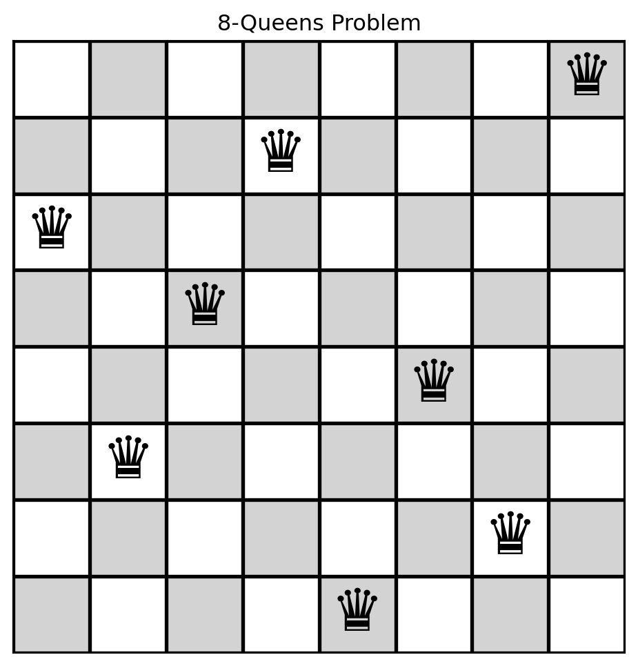
[7, 4, 2, 5, 2, 0, 3, 6] -> # of conflicts = 2
[7, 4, 2, 5, 3, 0, 3, 6] -> # of conflicts = 4
[7, 4, 2, 5, 4, 0, 3, 6] -> # of conflicts = 4
[7, 4, 2, 5, 5, 0, 3, 6] -> # of conflicts = 3
[7, 4, 2, 5, 6, 0, 3, 6] -> # of conflicts = 3
[7, 4, 2, 5, 7, 0, 3, 6] -> # of conflicts = 3
[7, 4, 2, 5, 1, 1, 3, 6] -> # of conflicts = 3
[7, 4, 2, 5, 1, 2, 3, 6] -> # of conflicts = 6
[7, 4, 2, 5, 1, 3, 3, 6] -> # of conflicts = 4
[7, 4, 2, 5, 1, 4, 3, 6] -> # of conflicts = 5
[7, 4, 2, 5, 1, 5, 3, 6] -> # of conflicts = 4
[7, 4, 2, 5, 1, 6, 3, 6] -> # of conflicts = 3
[7, 4, 2, 5, 1, 7, 3, 6] -> # of conflicts = 4
[7, 4, 2, 5, 1, 0, 0, 6] -> # of conflicts = 4
[7, 4, 2, 5, 1, 0, 1, 6] -> # of conflicts = 6
[7, 4, 2, 5, 1, 0, 2, 6] -> # of conflicts = 5
[7, 4, 2, 5, 1, 0, 4, 6] -> # of conflicts = 4
[7, 4, 2, 5, 1, 0, 5, 6] -> # of conflicts = 5
[7, 4, 2, 5, 1, 0, 6, 6] -> # of conflicts = 5
[7, 4, 2, 5, 1, 0, 7, 6] -> # of conflicts = 5
[7, 4, 2, 5, 1, 0, 3, 0] -> # of conflicts = 6
[7, 4, 2, 5, 1, 0, 3, 1] -> # of conflicts = 6
[7, 4, 2, 5, 1, 0, 3, 2] -> # of conflicts = 7
[7, 4, 2, 5, 1, 0, 3, 3] -> # of conflicts = 5
[7, 4, 2, 5, 1, 0, 3, 4] -> # of conflicts = 7
[7, 4, 2, 5, 1, 0, 3, 5] -> # of conflicts = 5
[7, 4, 2, 5, 1, 0, 3, 7] -> # of conflicts = 6

get_neighbors

def get_neighbors(state):

    """Generates neighboring states by swapping two rows."""

    neighbors = []
    n = len(state)

    for i in range(n):
        for j in range(i + 1, n):
            new_state = state[:]
            new_state[i], new_state[j] = new_state[j], new_state[i]
            neighbors.append(new_state)

    return neighbors

\(\frac{8 \times 7}{2} = 28\) neighbours

get_neighbors

etat = create_initial_state(8)
display_n_queens(etat, 5)

get_neighbors

print(initial_state_8)
for s in get_neighbors(initial_state_8):
  print(f"{s} -> # of conflicts = {calculate_conflicts(s)}")

[7, 4, 2, 5, 1, 0, 3, 6]
[4, 7, 2, 5, 1, 0, 3, 6] -> # of conflicts = 4
[2, 4, 7, 5, 1, 0, 3, 6] -> # of conflicts = 6
[5, 4, 2, 7, 1, 0, 3, 6] -> # of conflicts = 7
[1, 4, 2, 5, 7, 0, 3, 6] -> # of conflicts = 2
[0, 4, 2, 5, 1, 7, 3, 6] -> # of conflicts = 4
[3, 4, 2, 5, 1, 0, 7, 6] -> # of conflicts = 5
[6, 4, 2, 5, 1, 0, 3, 7] -> # of conflicts = 5
[7, 2, 4, 5, 1, 0, 3, 6] -> # of conflicts = 3
[7, 5, 2, 4, 1, 0, 3, 6] -> # of conflicts = 3
[7, 1, 2, 5, 4, 0, 3, 6] -> # of conflicts = 4
[7, 0, 2, 5, 1, 4, 3, 6] -> # of conflicts = 5
[7, 3, 2, 5, 1, 0, 4, 6] -> # of conflicts = 3
[7, 6, 2, 5, 1, 0, 3, 4] -> # of conflicts = 5
[7, 4, 5, 2, 1, 0, 3, 6] -> # of conflicts = 10
[7, 4, 1, 5, 2, 0, 3, 6] -> # of conflicts = 2
[7, 4, 0, 5, 1, 2, 3, 6] -> # of conflicts = 5
[7, 4, 3, 5, 1, 0, 2, 6] -> # of conflicts = 7
[7, 4, 6, 5, 1, 0, 3, 2] -> # of conflicts = 7
[7, 4, 2, 1, 5, 0, 3, 6] -> # of conflicts = 3
[7, 4, 2, 0, 1, 5, 3, 6] -> # of conflicts = 5
[7, 4, 2, 3, 1, 0, 5, 6] -> # of conflicts = 5
[7, 4, 2, 6, 1, 0, 3, 5] -> # of conflicts = 6
[7, 4, 2, 5, 0, 1, 3, 6] -> # of conflicts = 2
[7, 4, 2, 5, 3, 0, 1, 6] -> # of conflicts = 6
[7, 4, 2, 5, 6, 0, 3, 1] -> # of conflicts = 3
[7, 4, 2, 5, 1, 3, 0, 6] -> # of conflicts = 2
[7, 4, 2, 5, 1, 6, 3, 0] -> # of conflicts = 3
[7, 4, 2, 5, 1, 0, 6, 3] -> # of conflicts = 4

hill_climbing

def hill_climbing(current_state):

    current_conflicts = calculate_conflicts(current_state)

    while True:

        if current_conflicts == 0:
          return curent_state

        neighbors = get_neighbors(current_state)

        conflicts = [calculate_conflicts(neighbor) for neighbor in neighbors]

        if (min(conflicts)) > current_conflicts:
          return None # No improvement found, stuck at local minimum

        arg_best = np.argmin(conflicts)
        curent_state = neighbors[arg_best]
        current_conflicts = conflicts[arg_best]

The program above presents a major issue. What exactly is it?

It is important to note that, in this particular context, the problem is defined such that the sought solution is free of any conflict. However, in some optimization problems, the minimum value of the objective function is not predetermined.

The main issue is that the algorithm might enter an infinite loop if the condition min(conflicts == current_conflicts) is satisfied.

Two scenarios may arise: either the plateau is followed by an ascending slope, or it represents a local maximum. In the first case, the algorithm could potentially exit the plateau, although this is not guaranteed. To prevent infinite loops, it would be wise to implement an appropriate mechanism.

hill_climbing (take 2)

MAX_SIDE_MOVES = 100

def hill_climbing(current_state):

    conflicts_current_state = calculate_conflicts(current_state)
    side_moves = 0

    while True:

        if conflicts_current_state == 0:
          return current_state

        neighbors = get_neighbors(current_state)

        conflicts = [calculate_conflicts(voisin) for voisin in neighbors]

        if (min(conflicts)) > conflicts_current_state:
          return None  # No improvement, local maxima

        if (min(conflicts)) == conflicts_current_state:
          side_moves += 1  # Plateau

        if side_moves > MAX_SIDE_MOVES:
          return None

        arg_best = np.argmin(conflicts)
        current_state = neighbors[arg_best]
        conflicts_current_state = conflicts[arg_best]

Solve

random.seed(7)

solutions = 0

explored = set()
nb_duplicates = 0

for i in range(10):
  state = create_initial_state(8)

  new_state = hill_climbing(state)

  if (new_state != None):
    display_n_queens(new_state, 6)
    if tuple(new_state) in explored:
      nb_duplicates += 1
    solutions += 1

print(f"10 runs, number of solutions = {solutions}, {nb_duplicates} duplicate(s)")

10 runs, number of solutions = 9, 0 duplicate(s)

Solve (2)

random.seed(7)

solutions = 0

explored = set()
nb_duplicates = 0

nb_runs = 1000

for i in range(nb_runs):

  state = create_initial_state(8)

  new_state = hill_climbing(state)

  if (new_state != None):

    if tuple(new_state) in explored:
      nb_duplicates += 1
    else:
      explored.add(tuple(new_state))

    solutions += 1

print(f"{nb_runs} runs, number of solutions = {solutions}, {len(explored)} unique solutions")

1000 runs, number of solutions = 704, 92 unique solutions

Solve 40-Queens

\(40! = 8.1591528325 \times 10^{47}\)

import time

start_time = time.time()  # Record the start time

random.seed(7)

solutions = 0

explored = set()
nb_duplicates = 0

nb_runs = 10

for i in range(nb_runs):

  state = create_initial_state(40)

  new_state = hill_climbing(state)

  if (new_state != None):

    if tuple(new_state) in explored:
      nb_duplicates += 1
    else:
      explored.add(tuple(new_state))

    solutions += 1

print(f"{nb_runs} runs, number of solutions = {solutions}, {len(explored)} unique solutions")

one_board = next(iter(explored))
display_n_queens(one_board, 12)

end_time = time.time()  # Record the end time
elapsed_time = end_time - start_time  # Calculate the elapsed time

print(f"Elapsed time: {elapsed_time:.4f} seconds")

10 runs, number of solutions = 6, 6 unique solutions

Elapsed time: 22.2250 seconds

Iterations and Side Moves

MAX_SIDE_MOVES = 100

def hill_climbing_counts(current_state):

    conflicts_current_state = calculate_conflicts(current_state)
    side_moves = 0
    iterations = 0

    while True:

        if conflicts_current_state == 0:
          return (iterations, side_moves, current_state)

        iterations += 1

        neighbors = get_neighbors(current_state)

        conflicts = [calculate_conflicts(voisin) for voisin in neighbors]

        if (min(conflicts)) > conflicts_current_state:
          return (iterations, side_moves, None)  # No improvement, local maxima

        if (min(conflicts)) == conflicts_current_state:
          side_moves += 1  # Plateau

        if side_moves > MAX_SIDE_MOVES:
          return (iterations, side_moves, None)

        arg_best = np.argmin(conflicts)
        current_state = neighbors[arg_best]
        conflicts_current_state = conflicts[arg_best]

random.seed(7)

solutions = 0

explored = set()
nb_duplicates = 0

nb_runs = 1000

iterations = []
sides = []

iterations_none = []
sides_none = []

for i in range(nb_runs):

  state = create_initial_state(8)

  (i, s, new_state) = hill_climbing_counts(state)

  if new_state != None:
    iterations.append(i)
    sides.append(s)
  else:
    iterations_none.append(i)
    sides_none.append(s)

  if new_state != None:

    if tuple(new_state) in explored:
      nb_duplicates += 1
    else:
      explored.add(tuple(new_state))

    solutions += 1

print(f"{nb_runs} runs, number of solutions = {solutions}, {len(explored)} unique solutions")

1000 runs, number of solutions = 704, 92 unique solutions

Iterations and Side Moves

import seaborn as sns
import matplotlib.pyplot as plt

# Configurer la structure des sous-graphiques
fig, axes = plt.subplots(1, 2, figsize=(14, 6), sharey=True)

# Tracer l'histogramme pour `iterations`
sns.histplot(iterations, kde=True, color='green', ax=axes[0], edgecolor='black')
axes[0].set_title("Histogram of Iterations")
axes[0].set_xlabel("Iterations")
axes[0].set_ylabel("Frequency")

# Tracer l'histogramme pour `sides`
sns.histplot(sides, kde=True, color='blue', ax=axes[1], edgecolor='black')

axes[1].set_title("Histogram of Side Moves")
axes[1].set_xlabel("# Side Moves")

# Afficher le graphique
plt.legend()
plt.tight_layout()
plt.show()

Iterations and Side Moves

20-Queens

random.seed(7)

solutions = 0

explored = set()
nb_duplicates = 0

nb_runs = 1000

iterations = []
sides = []

iterations_none = []
sides_none = []

for i in range(nb_runs):

  state = create_initial_state(20)

  (i, s, new_state) = hill_climbing_counts(state)

  if new_state != None:
    iterations.append(i)
    sides.append(s)
  else:
    iterations_none.append(i)
    sides_none.append(s)

  if new_state != None:

    if tuple(new_state) in explored:
      nb_duplicates += 1
    else:
      explored.add(tuple(new_state))

    solutions += 1

print(f"{nb_runs} runs, number of solutions = {solutions}, {len(explored)} unique solutions")

1000 runs, number of solutions = 566, 566 unique solutions

import seaborn as sns
import matplotlib.pyplot as plt

# Configurer la structure des sous-graphiques
fig, axes = plt.subplots(1, 2, figsize=(14, 6), sharey=True)

# Tracer l'histogramme pour `iterations`
sns.histplot(iterations, kde=True, color='green', ax=axes[0], edgecolor='black')
axes[0].set_title("Histogram of Iterations")
axes[0].set_xlabel("Iterations")
axes[0].set_ylabel("Frequency")

# Tracer l'histogramme pour `sides`
sns.histplot(sides, kde=True, color='blue', ax=axes[1], edgecolor='black')

axes[1].set_title("Histogram of Side Moves")
axes[1].set_xlabel("# Side Moves")

# Afficher le graphique
plt.legend()
plt.tight_layout()
plt.show()

20-Queens

Russell & Norvig

• Hill climbing gets stuck 86% of the time.
  • Successful attempts average 4 steps to a solution.
• Permitting 100 lateral moves boosts success rate from 14% to 94%.
• The problem space comprises \(8^8 = 16,777,216\) states.
  • Implementation from Russell & Norvig

In the implementation I proposed, there do not appear to be any local minima. However, this requires further verification.

Has many variants, including random-restart hill climbing.

Escaping a Local Optimum

What mechanisms would enable the hill climbing algorithm to escape from a local optimum, whether it be a local minimum or maximum?

It needs to accept going downhill.

A random walk approach, which disregards the value of the objective function, could theoretically locate the global maximum. However, this method is highly impractical due to its extreme inefficiency.

Remark

Assume the optimization problem is a minimization task, where the goal is to find a solution with the minimum cost.

Downhill, gradient descent.

Simulated Annealing

Definition

Simulated annealing is an optimization algorithm inspired by the annealing process in metallurgy. It probabilistically explores the solution space by allowing occasional uphill moves, which helps escape local optima. The algorithm gradually reduces the probability of accepting worse solutions by lowering a “temperature” parameter, ultimately converging towards an optimal or near-optimal solution.

Annealing

(Russell and Norvig 2020, 114)

In metallurgy, annealing is the process used to temper or harden metals and glass by heating them to a high temperature and then gradually cooling them, thus allowing the material to reach a low-energy crystalline state.

The solid is heated to its melting point, causing the particles to become randomly distributed.

Subsequently, the material is gradually cooled, allowing the particles to reorganize into a low-energy state.

Algorithm

1. This algorithm resembles hill climbing but differs by randomly selecting the next state rather than choosing the optimal move.

2. If the move results in a lower objective function value, it is accepted unconditionally.

3. Otherwise, acceptance is probabilistic, contingent on both \(\Delta E\) and \(T\).

Attribution: (Russell and Norvig 2020, 115)

Varying \(\Delta E\)

import numpy as np
import matplotlib.pyplot as plt

# Define a fixed temperature, T
T = 1.0  # You can adjust this value as needed

# Define a range of energy changes, ΔE
delta_E = np.linspace(0, 5, 500)

# Compute the function e^(-ΔE/T)
y = np.exp(-delta_E / T)

# Plot the function
plt.figure(figsize=(8, 5))
plt.plot(delta_E, y, label=r'$e^{-\frac{\Delta E}{T}}$', color='blue')
plt.title(r'Plot of $e^{-\Delta E / T}$')
plt.xlabel(r'Energy Change ($\Delta E$)')
plt.ylabel(r'$e^{-\Delta E / T}$')
plt.ylim(0, 1.1)
plt.xlim(0, 5)
plt.grid(True)
plt.legend()
plt.show()

Moves resulting in significant negative changes (worse) to the objective function are less likely to be accepted.

Varying the temperature, \(T\)

import numpy as np
import matplotlib.pyplot as plt

# Define the energy change, ΔE
delta_E = 0.1  # You can adjust this value as needed

# Define a range of temperatures, T
T = np.linspace(0.1, 5, 500)  # Avoid T=0 to prevent division by zero

# Compute the function e^(-ΔE/T)
y = np.exp(-delta_E / T)

# Plot the function
plt.figure(figsize=(8, 5))
plt.plot(T, y, label=r'$e^{-\frac{\Delta E}{T}}$', color='blue')
plt.title(r'Plot of $e^{-\Delta E / T}$')
plt.xlabel('Temperature (T)')
plt.ylabel(r'$e^{-\Delta E / T}$')
plt.ylim(0, 1.1)
plt.xlim(0, 5)
plt.grid(True)
plt.legend()
plt.show()

For a fixed \(\Delta E\) (here \(0.1\)), changes are more likely to be accepted whe \(T\) is high, at the start of the algorithm.

Varying the temperature and \(\Delta E\)

import numpy as np
import matplotlib.pyplot as plt

# Define a range of temperatures, T
T = np.linspace(0.1, 5, 500)  # Avoid T=0 to prevent division by zero

# Define specific values for energy change, ΔE
delta_E_values = [0.001, 0.01, 0.1, 1.0, 2.0]

# Plot the function for each ΔE
plt.figure(figsize=(10, 6))
for delta_E in delta_E_values:
    y = np.exp(-delta_E / T)
    plt.plot(T, y, label=r'$\Delta E = {:.3f}$'.format(delta_E))

# Customize the plot
plt.title(r'Plot of $e^{-\Delta E / T}$ for Different $\Delta E$ Values')
plt.xlabel('Temperature (T)')
plt.ylabel(r'$e^{-\Delta E / T}$')
plt.ylim(0, 1.1)
plt.xlim(0, 5)
plt.grid(True)
plt.legend()
plt.show()

Bad moves are more likely to be accepted at the start when \(T\) is high, and less likely as \(T\) decreases.

Varying the temperature and \(\Delta E\)

import { Inputs, Plot } from "@observablehq/plot"

viewof deltaE = Inputs.range([0.01, 100], {step: 0.01, value: 0.1, label: "ΔE", width: 300})

T_values = Array.from({length: 1000}, (_, i) => (i + 1) * 0.1)

function computeData(deltaE) {
  return T_values.map(T => ({
    T: T,
    value: Math.exp(-deltaE / T)
  }))
}

data = computeData(deltaE)

Plot.plot({
  marks: [
    Plot.line(data, {
      x: "T", 
      y: "value", 
      stroke: "steelblue", 
      strokeWidth: 2
    }),
    Plot.ruleX([0], {stroke: "black"}), // X-axis line
    Plot.ruleY([0], {stroke: "black"})  // Y-axis line
  ]
})

Using Observable JS.

Theory

(Russell and Norvig 2020, 114)

If the schedule lowers \(T\) to 0 slowly enough, then a property of the Boltzmann (aka Gibbs) distribution, \(e^{\frac{\Delta E}{T}}\), is that all the probability is concentrated on the global maxima, which the algorithm will find with probability approaching 1.

See also: Laarhoven and Aarts (1987), Aarts and Korst (1989)

Definition

The Travelling Salesman Problem (TSP) is a classic optimization problem that seeks the shortest possible route for a salesman to visit a set of cities, returning to the origin city, while visiting each city exactly once.

The challenge lies in determining the most efficient path, especially as the number of cities increases, due to the combinatorial explosion of possible routes.

Traveling Salesman

# Ensure we always generate the same coordinates

np.random.seed(42)

# Generate random coordinates for the cities

num_cities = 20
coordinates = np.random.rand(num_cities, 2) * 100

# Calculate the distance matrix

distance_matrix = np.sqrt(((coordinates[:, np.newaxis] - coordinates[np.newaxis, :]) ** 2).sum(axis=2))

import matplotlib.pyplot as plt

def plot_cities(coordinates, title="Cities of the Traveling Salesman Problem"):

    """
    Plot the given coordinates representing the cities.
    
    Parameters:
    - coordinates: A 2D NumPy array of shape (n, 2) representing the (x, y) coordinates.
    - title: Title of the plot.
    """

    # Extract x and y coordinates
    x = coordinates[:, 0]
    y = coordinates[:, 1]

    plt.figure(figsize=(6, 6))

    # Plot the cities as red points
    plt.scatter(x, y, c='red', zorder=2)

    # Annotate the cities with their indices
    for i, (xi, yi) in enumerate(zip(x, y)):
        plt.annotate(str(i + 1), (xi, yi), textcoords="offset points", xytext=(0, 5), ha='center')

    # Set the title and labels
    plt.title(title)
    plt.xlabel('X Coordinate')
    plt.ylabel('Y Coordinate')
    plt.grid(True)
    plt.axis('equal')  # Equal scaling for x and y axes
    plt.show()

plot_cities(distance_matrix)

Traveling Salesman

How to Represent a Solution?

We will use a list where each element represents the index of a city, and the order of elements indicates the sequence of city visits.

Random Solution

def plot_tsp_path(coordinates, path=None, title="Travelling Salesman Problem"):

    """
    Plots the given coordinates and optionally a path for the TSP.
    
    Parameters:
    - coordinates: A 2D NumPy array of shape (n, 2) representing the (x, y) coordinates.
    - path: A list or array of indices representing the order of cities to visit. If None, the nodes are connected in input order.
    - title: Title of the plot.
    """

    # Extract x and y coordinates
    x = coordinates[:, 0]
    y = coordinates[:, 1]

    plt.figure(figsize=(6, 6))

    # If a path is given, rearrange the coordinates
    if path is not None:
        x = x[path]
        y = y[path]
    
    # Plot the nodes
    plt.scatter(x, y, c='red', zorder=2)

    # Annotate the nodes with their indices
    for i, (xi, yi) in enumerate(zip(x, y)):
        plt.annotate(str(i + 1), (xi, yi), textcoords="offset points", xytext=(0, 5), ha='center')

    # Plot the path
    plt.plot(x, y, 'b-', zorder=1)

    # If a path is provided, connect the last point to the first to complete the tour
    if path is not None:
        plt.plot([x[-1], x[0]], [y[-1], y[0]], 'b-', zorder=1)

    # Set the title and labels
    plt.title(title)
    plt.xlabel('X Coordinate')
    plt.ylabel('Y Coordinate')
    plt.grid(True)
    plt.axis('equal')  # Equal scale for x and y axes
    plt.show()

num_cities = len(distance_matrix)
current_route = np.arange(num_cities)
np.random.shuffle(current_route)
plot_tsp_path(distance_matrix, current_route)

Calculate the Total Distance

# Function to calculate the total distance of a given route

def calculate_total_distance(route, distance_matrix):

    total_distance = 0

    for i in range(len(route) - 1):
        total_distance += distance_matrix[route[i], route[i + 1]]

    total_distance += distance_matrix[route[-1], route[0]]  # Back to start

    return total_distance

Neighborhood

plot_tsp_path(distance_matrix,current_route)

How to generate a neighboring solution?

Generating a Neighboring Solution

How to generate a neighboring solution?

Swap Two Cities

• Description: Select two cities at random and swap their positions.
• Pros: Simple and effective for exploring nearby solutions.
• Cons: Change may be too small, potentially slowing down convergence.

Reverse Segment

• Description: Select two indices and reverse the segment between them.
• Pros: More effective at finding shorter paths compared to simple swaps.
• Cons: Can still be computationally expensive as the number of cities increases.

Remove & Reconnect

• Description: Removes three edges from the route and reconnects the segments in the best possible way. This can generate up to 7 different routes.
• Pros: Provides more extensive changes and can escape local optima more effectively than 2-opt.
• Cons: More complex and computationally expensive to implement.

Insertion Move

• Description: Select a city and move it to a different position in the route.
• Pros: Offers a balance between small and large changes, making it useful for fine-tuning solutions.
• Cons: May require more iterations to converge to an optimal solution.

Shuffle Subset

• Description: Select a subset of cities in the route and randomly shuffle their order.
• Pros: Introduces larger changes and can help escape local minima.
• Cons: Can lead to less efficient routes if not handled carefully.

Generating a Neighboring Solution

# Function to generate a random neighboring solution

def get_neighbor(route):

    a, b = np.random.randint(0, len(route), size=2)

    if a > b:
        a, b = b, a

    new_route = route.copy()
    new_route[a:b+1] = new_route[a:b+1][::-1]  # Reverse the segment between a and b
    
    return new_route

simulated_annealing

def simulated_annealing(distance_matrix, initial_temp, cooling_rate, max_iterations):

    num_cities = len(distance_matrix)
    current_route = np.arange(num_cities)
    np.random.shuffle(current_route)
    current_cost = calculate_total_distance(current_route, distance_matrix)
    
    best_route = current_route.copy()
    best_cost = current_cost

    temperature = initial_temp

    for iteration in range(max_iterations):

        neighbor_route = get_neighbor(current_route)
        neighbor_cost = calculate_total_distance(neighbor_route, distance_matrix)
        
        # Accept the neighbor if it is better, or with a probability if it is worse.

        delta_E = neighbor_cost - current_cost

        if neighbor_cost < current_cost or np.random.rand() < np.exp(-(delta_E)/temperature):
            current_route = neighbor_route
            current_cost = neighbor_cost

            if current_cost < best_cost:
                best_route = current_route.copy()
                best_cost = current_cost

        # Cool down the temperature
        temperature *= cooling_rate

    return best_route, best_cost, temperatures, costs

Remarks

• As \(t \to \infty\), the algorithm exhibits behavior characteristic of a random walk. During this phase, any neighboring state, regardless of whether it improves the objective function, is accepted. This facilitates exploration and occurs at the start of the algorithm’s execution.

Remarks

• Conversely, as \(t \to 0\), the algorithm behaves like hill climbing. In this phase, only those states that enhance the objective function’s value are accepted, ensuring that the algorithm consistently moves towards optimal solutions—specifically, towards lower values in minimization problems. This phase emphasizes the exploitation of promising solutions and occurs towards the algorithm’s conclusion.

1. Exploration:
   • Exploration involves searching through a broad area of the search space to discover new possibilities, solutions, or information. The goal of exploration is to gather a diverse set of data points or solutions that could potentially lead to finding better global optima. It prevents the search process from getting trapped in local optima by encouraging the consideration of less-visited or unexplored regions of the search space.
   • In algorithms, exploration can be implemented by introducing randomness, trying new or less-promising paths, or using strategies like simulated annealing or genetic algorithms that encourage diversity.
2. Exploitation:
   • Exploitation focuses on leveraging known information to refine and improve existing solutions. It involves concentrating the search effort around areas believed to contain high-quality solutions based on prior knowledge or experience. The goal is to optimize and fine-tune these solutions to achieve the best possible outcome in those regions.
   • In algorithms, exploitation can be seen in strategies like hill climbing, gradient ascent/descent, or greedy algorithms, where the search is focused on local improvement and making incremental gains.

See also: Properties of Simulated Annealing - Georgia Tech - Machine Learning. Udacity video (4m 10s). Posted on 2015-02-23.

Example

# Ensuring reproducibility
np.random.seed(42)

# Generate random coordinates for cities
num_cities = 20
coordinates = np.random.rand(num_cities, 2) * 100

# Calculate distance matrix
distance_matrix = np.sqrt(((coordinates[:, np.newaxis] - coordinates[np.newaxis, :]) ** 2).sum(axis=2))

# Run simulated annealing

initial_temp = 15
cooling_rate = 0.995
max_iterations = 1000

Held–Karp Algorithm

• Introduced: 1962 by Held, Karp, and independently by Bellman.
• Problem: Solves the Traveling Salesman Problem (TSP) using dynamic programming.
• Time Complexity: \(\Theta(2^n n^2)\).
• Space Complexity: \(\Theta(2^n n)\).
• Efficiency: Better than brute-force \(\Theta(n!)\), yet still exponential.

Held–Karp Algorithm

from itertools import combinations
import numpy as np

def held_karp(distance_matrix):
    # Number of cities
    n = len(distance_matrix)

    # DP table: dp[subset][last_visited] = minimum cost to reach `last_visited` with `subset` of cities visited
    dp = {}

    # Initialize the DP table with the distances from the starting point (city 0)
    for i in range(1, n):
        dp[(1 << i, i)] = distance_matrix[0][i]

    # Iterate over all subset sizes
    for subset_size in range(2, n):
        for subset in combinations(range(1, n), subset_size):
            # Bitmask of the subset, excluding the starting city
            subset_mask = sum(1 << i for i in subset)
            for last in subset:
                # Update the DP table with the minimum cost for this subset and last city
                prev_subset_mask = subset_mask & ~(1 << last)
                dp[(subset_mask, last)] = min(
                    dp[(prev_subset_mask, k)] + distance_matrix[k][last]
                    for k in subset if k != last
                )

    # Find the minimum cost to complete the tour back to the starting point (city 0)
    full_mask = (1 << n) - 2  # All cities visited except starting city
    return min(dp[(full_mask, last)] + distance_matrix[last][0] for last in range(1, n))

# Example usage with a sample distance matrix
# distance_matrix = [
#     [0, 10, 15, 20],
#     [10, 0, 35, 25],
#     [15, 35, 0, 30],
#     [20, 25, 30, 0]
# ]
min_cost = held_karp(distance_matrix)
print(f"Using Held–Karp to find the minimum cost of TSP tour: {min_cost:.2f}")

Using Held–Karp to find the minimum cost of TSP tour: 386.43

Held and Karp (1962) and Bellman (1962)

Execution

# Simulated Annealing function

def simulated_annealing(distance_matrix, initial_temp, cooling_rate, max_iterations):
    num_cities = len(distance_matrix)
    current_route = np.arange(num_cities)
    np.random.shuffle(current_route)
    current_cost = calculate_total_distance(current_route, distance_matrix)
    
    best_route = current_route.copy()
    best_cost = current_cost

    temperatures = []
    costs = []

    temperature = initial_temp

    # Collect intermediate solutions
    intermediate_solutions = []
    for iteration in range(max_iterations):
        neighbor_route = get_neighbor(current_route)
        neighbor_cost = calculate_total_distance(neighbor_route, distance_matrix)
        
        # Accept neighbor if it's better, or with a probability if it's worse
        if neighbor_cost < current_cost or np.random.rand() < np.exp(-(neighbor_cost - current_cost) / temperature):
            current_route = neighbor_route
            current_cost = neighbor_cost

            if current_cost < best_cost:
                best_route = current_route.copy()
                best_cost = current_cost

        # Store temperature and cost for plotting
        temperatures.append(temperature)
        costs.append(current_cost)

        # Cool down the temperature
        temperature *= cooling_rate

        # Collect intermediate solutions at regular intervals
        if iteration % (max_iterations // 10) == 0:
            intermediate_solutions.append((current_route.copy(), current_cost))

    # Plot 10 intermediate solutions in a 4x5 grid
    fig, axes = plt.subplots(2, 5, figsize=(12, 6))
    axes = axes.flatten()
    for idx, (route, cost) in enumerate(intermediate_solutions):
        ax = axes[idx]
        ax.scatter(*zip(*coordinates), c='red', marker='o')
        ax.plot(*zip(*coordinates[route]), 'b-', alpha=0.6)
        ax.set_title(f"Iteration: {idx*100} - Cost: {cost:.0f}")
        ax.axis('off')  # Turn off the axes for a cleaner look
    plt.tight_layout()
    plt.show()

    return best_route, best_cost, temperatures, costs


best_route, best_cost, temperatures, costs = simulated_annealing(distance_matrix, initial_temp, cooling_rate, max_iterations)

When I initially published these slides, the selected initial temperature of 1000 was excessively high relative to the objective function’s cost. By adjusting the initial temperature to 15, we achieve a more effective balance between exploration and exploitation.

Due to the snapshots being captured every 100 iterations, the increases in cost are not visible. This is illustrated on the “Temperature and Cost” slide.

Best Route

# Plot the final best route
plt.figure(figsize=(5, 5))
plt.scatter(*zip(*coordinates), c='red', marker='o')
plt.plot(*zip(*coordinates[best_route]), 'b-', alpha=0.6)
plt.title(f"Best Route - Cost: {best_cost:.2f}")
plt.show()

We have found an optimal tour!

Temperature and Cost

# Plot temperature and cost graphs
plt.figure(figsize=(12, 5))

plt.subplot(1, 2, 1)
plt.plot(temperatures)
plt.title("Temperature Over Iterations")
plt.xlabel("Iteration")
plt.ylabel("Temperature")

plt.subplot(1, 2, 2)
plt.plot(costs)
plt.title("Cost Over Iterations")
plt.xlabel("Iteration")
plt.ylabel("Cost")

plt.tight_layout()
plt.show()

Swapping Neighbors

• Description: Select two cities at random, swap their positions.
• Pros: Simple and effective for exploring nearby solutions.
• Cons: Change may be too small, potentially slowing down convergence.

def get_neighbor_swap(route):
    a, b = np.random.randint(0, len(route), size=2)
    new_route = route.copy()
    new_route[a], new_route[b] = new_route[b], new_route[a]
    return new_route

Execution

# Plot the final best route
get_neighbor = get_neighbor_swap

best_route, best_cost, temperatures, costs = simulated_annealing(distance_matrix, initial_temp, cooling_rate, max_iterations)

Best Route

# Plot the final best route
plt.figure(figsize=(5, 5))
plt.scatter(*zip(*coordinates), c='red', marker='o')
plt.plot(*zip(*coordinates[best_route]), 'b-', alpha=0.6)
plt.title(f"Best Route - Cost: {best_cost:.2f}")
plt.show()

In this specific instance and for the given problem, reverse segment (cost = 386.43) was more effective compared to swapping neighbors (cost = 430.03).

Temperature and Cost

# Plot temperature and cost graphs
plt.figure(figsize=(12, 5))

plt.subplot(1, 2, 1)
plt.plot(temperatures)
plt.title("Temperature Over Iterations")
plt.xlabel("Iteration")
plt.ylabel("Temperature")

plt.subplot(1, 2, 2)
plt.plot(costs)
plt.title("Cost Over Iterations")
plt.xlabel("Iteration")
plt.ylabel("Cost")

plt.tight_layout()
plt.show()

Selecting a Neighborhood Strategy

• Simple Moves (Swap, Insertion): Effective for initial exploration; risk of local optima entrapment.

• Complex Moves: Enhance capability to escape local optima and accelerate convergence; entail higher computational expense.

• Hybrid Approaches: Integrate diverse strategies for neighborhood generation. Employ simple moves initially, transitioning to complex ones as convergence progresses.

Initial Temperature

Influence: Since the probability of accepting a new state is given by \(e^{-\frac{\Delta E}{T}}\), the selection of the initial temperature is directly influenced by \(\Delta E\) and consequently by the objective function value for a random state, \(f(s)\).

Initial Temperature

• Example Problems: Consider two scenarios: problem \(a\) with \(f(a) = 1,000\) and problem \(b\) with \(f(b) = 100\).

• Energy Difference: Accepting a state that is 10% worse results in energy differences \(\Delta E = 0.1 \cdot f(a) = 100\) for problem \(a\) and \(\Delta E = 0.1 \cdot f(b) = 10\) for problem \(b\).

• Acceptance Probability: To accept such state 60% of the time, set \(e^{-\frac{\Delta E}{T}} = 0.6\). Solving for \(T\) yields initial temperatures of approximately \(T \approx 195.8\) for problem \(a\) and \(T \approx 19.58\) for problem \(b\).

Initial Temperature

A popular approach is to set the initial temperature so that a significant portion of moves (often around 60-80%) are accepted.

This can be done by running a preliminary phase where the temperature is adjusted until the acceptance ratio stabilizes within this range.

Ben-Ameur (2004) suggests a more rigorous mathematical methodology.

Cooling Strategies

In simulated annealing, cooling down is essential for managing algorithm convergence. The cooling schedule dictates the rate at which the temperature decreases, affecting the algorithm’s capacity to escape local optima and converge towards a near-optimal solution.

Nourani and Andresen (1998) and Alex, Simon, and Samuel (2017)

Linear Cooling

• Description: The temperature decreases linearly with each iteration.
• Formula: \(T = T_0 - \alpha \cdot k\)
  • \(T_0\): Initial temperature
  • \(\alpha\): A constant decrement
  • \(k\): Current iteration
• Pros: Simple to implement and understand.
• Cons: Often leads to premature convergence because the temperature decreases too quickly.

temperature = initial_temp - alpha * iteration

Geometric (Exponential) Cooling

• Description: The temperature decreases exponentially with each iteration.
• Formula: \(T = T_0 \cdot \alpha^k\)
  • \(\alpha\): Cooling rate, typically between 0.8 and 0.99
  • \(k\): Current iteration
• Pros: Widely used due to its simplicity and effectiveness.
• Cons: The choice of \(\alpha\) is critical; if it’s too small, the temperature drops too fast, and if it’s too large, convergence can be slow.

temperature = initial_temp * (cooling_rate ** iteration)

Logarithmic Cooling

• Description: The temperature decreases slowly following a logarithmic function.
• Formula: \(T = \frac{\alpha \cdot T_0}{\log(1+k)}\)
  • \(\alpha\): A scaling constant
  • \(k\): Current iteration
• Pros: Provides a slower cooling rate, which is useful for problems that require extensive exploration of the solution space.
• Cons: Convergence can be very slow, requiring many iterations.

temperature = alpha * initial_temp / (np.log(1 + iteration))

Inverse Cooling

• Description: The temperature decreases as an inverse function of the iteration number.
• Formula: \(T = \frac{T_0}{1+\alpha \cdot K}\)
  • \(\alpha\): A scaling constant
  • \(k\): Current iteration
• Pros: Allows for a more controlled cooling process, balancing exploration and exploitation.
• Cons: May require careful tuning of \(\alpha\) to be effective.

temperature = initial_temp / (1 + alpha * iteration)

Adaptive Cooling

• Description: The cooling schedule is adjusted dynamically based on the performance of the algorithm.
• Strategy: If the algorithm is not making significant progress, the cooling rate may be slowed down. Conversely, if progress is steady, the cooling rate can be increased.
• Pros: More flexible and can adapt to the characteristics of the problem.
• Cons: More complex to implement and requires careful design to avoid instability.

if no_significant_change_in_cost:
    temperature *= 0.99  # Slow down cooling
else:
    temperature *= 0.95  # Speed up cooling

Cooling Schedule - Summary

# Constants
initial_temp = 100
alpha = 0.995
iterations = np.arange(0, 1001)

# Cooling strategies
def exponential_cooling(initial_temp, alpha, iteration):
    return initial_temp * (alpha ** iteration)

def linear_cooling(initial_temp, alpha, iteration):
    return max(0, initial_temp - alpha * iteration)

def logarithmic_cooling(initial_temp, alpha, iteration):
    return min(initial_temp, alpha * initial_temp / (np.log(1 + iteration) + 10e-9))

def inverse_cooling(initial_temp, alpha, iteration):
    return initial_temp / (1 + alpha * iteration)

# Calculate temperatures
linear_temps = [linear_cooling(initial_temp, alpha, i) for i in iterations]
exponential_temps = [exponential_cooling(initial_temp, alpha, i) for i in iterations]
logarithmic_temps = [logarithmic_cooling(initial_temp, alpha, i) for i in iterations]
inverse_temps = [inverse_cooling(initial_temp, alpha, i) for i in iterations]

# Plotting
plt.figure(figsize=(8, 6))
plt.plot(iterations, exponential_temps, label='Exponential Cooling')
plt.plot(iterations, linear_temps, label='Linear Cooling')
plt.plot(iterations, logarithmic_temps, label='Logarithmic Cooling')
plt.plot(iterations, inverse_temps, label='Inverse Cooling')
plt.xlabel('Iteration')
plt.ylabel('Temperature')
plt.title(r'Cooling Strategies ($\alpha = 0.995$)')
plt.legend()
plt.grid(True)
plt.show()

See also: Effective Simulated Annealing with Python by Nathan A. Rooy.

Choosing the Right Cooling Schedule

• Problem-Specific: The choice of cooling schedule often depends on the characteristics of the problem being solved. Some problems benefit from a slower cooling rate, while others may need faster convergence.

• Experimentation: It’s common to experiment with different strategies and parameters to find the best balance between exploration (searching broadly) and exploitation (refining the current best solutions).

Conclusion

After applying simulated annealing, a local search method such as hill climbing can be used to refine the solution.

Simulated annealing is effective for exploring the solution space and avoiding local minima, while local search focuses on the exploration of neighboring solutions.

Simulated Annealing Visualization

Attribution: ComputationalScientist, Posted on 2018-01-06.

Prologue

Summary

• Local search algorithms focus on finding goal states by moving between neighboring states without tracking paths.
• The hill-climbing algorithm seeks the highest-valued neighbor but can get stuck in local maxima or plateaus.
• Effective state representation, such as using permutations in the 8-Queens problem, avoids illegal placements and improves performance.
• Simulated annealing allows occasional uphill moves to escape local optima, controlled by a decreasing temperature parameter.
• The acceptance probability in simulated annealing decreases as temperature lowers and energy difference increases.
• Simulated annealing effectively solves complex problems like the Travelling Salesman Problem by probabilistically exploring the solution space.

Further Readings

“The overall SA [simulated annealing] methodology is then deployed in detail on a real-life application: a large-scale aircraft trajectory planning problem involving nearly 30,000 flights at the European continental scale.”

(Gendreau and Potvin 2019, chap. 1)

Did you know that you can freely access the entire collection of books from Springer? By using a device connected to a uOttawa IP address and visiting Springer Link, you have the ability to download books in either PDF or EPUB format.

The book is co-edited by Jean-Yves Potvin and Michel Gendreau. Jean-Yves Potvin serves as a professor at the Université de Montréal, while Michel Gendreau holds a professorship at École Polytechnique de Montréal.

Gendreau and Potvin (2019), access via Springer Link.

Next lecture

• We will discuss population-based algorithms.

References

Aarts, E. H. L., and J. H. M. Korst. 1989. Simulated Annealing and Boltzmann Machines : A Stochastic Approach to Combinatorial Optimization and Neural Computing. Wiley-Interscience Series in Discrete Mathematics and Optimization. Wiley.

Alex, Kwaku Peprah, Kojo Appiah Simon, and Kwame Amponsah Samuel. 2017. “An Optimal Cooling Schedule Using a Simulated Annealing Based Approach.” Applied Mathematics 08 (08): 1195–1210. https://doi.org/10.4236/am.2017.88090.

Bellman, Richard. 1962. “Dynamic Programming Treatment of the Travelling Salesman Problem.” Journal of the ACM (JACM) 9 (1): 61–63. https://doi.org/10.1145/321105.321111.

Ben-Ameur, Walid. 2004. “Computing the Initial Temperature of Simulated Annealing.” Computational Optimization and Applications 29 (3): 369–85. https://doi.org/10.1023/b:coap.0000044187.23143.bd.

Gendreau, M., and J. Y. Potvin. 2019. Handbook of Metaheuristics. International Series in Operations Research & Management Science. Springer International Publishing. https://books.google.com.ag/books?id=RbfFwQEACAAJ.

Held, Michael, and Richard M. Karp. 1962. “A Dynamic Programming Approach to Sequencing Problems.” Journal of the Society for Industrial and Applied Mathematics 10 (1): 196–210. https://doi.org/10.1137/0110015.

Laarhoven, P. J. M., and E. H. L. Aarts. 1987. Simulated Annealing: Theory and Applications. USA: Kluwer Academic Publishers.

Nourani, Yaghout, and Bjarne Andresen. 1998. “A Comparison of Simulated Annealing Cooling Strategies.” Journal of Physics A: Mathematical and General 31 (41): 8373.

Russell, Stuart, and Peter Norvig. 2020. Artificial Intelligence: A Modern Approach. 4th ed. Pearson. http://aima.cs.berkeley.edu/.

Marcel Turcotte

Marcel.Turcotte@uOttawa.ca

School of Electrical Engineering and Computer Science (EECS)

University of Ottawa