Explain the concept and key steps of Monte Carlo Tree Search (MCTS).
Compare MCTS with other search algorithms like BFS, DFS, A*, Simulated Annealing, and Genetic Algorithms.
Analyze how MCTS balances exploration and exploitation using the UCB1 formula.
Implement MCTS in practical applications such as Tic-Tac-Toe.
Introduction
Monte Carlo Tree Search (MCTS)
In the introductory lecture on state space search, I used Monte Carlo Tree Search (MCTS), a key component of AlphaGo, to exemplify the role of search algorithms in reasoning.
Today, we conclude this series by examining the implementation details of this algorithm.
Applications
De novo drug design
Electronic circuit routing
Load monitoring in smart grids
Lane keeping and overtaking tasks
Motion planning in autonomous driving
Even solving the travelling salesman problem
Applications (continued)
See also Besta et al. (2025) on the role of MTCS in Reasoning Language Models (RLMs).
Historical Notes
2008: the algorithm is introduced in the context of AI game(Chaslot et al. 2008)
2016: the algorithm is combined with deep neural networks to create AlphaGo(Silver et al. 2016)
Definition
A Monte Carlo algorithm is a computational method that uses random sampling to obtain numerical results, often used for optimization, numerical integration, and probability distribution estimation.
It is characterized by its ability to handle complex problems with probabilistic solutions, trading exactness for efficiency and scalability.
Algorithm
For a specified number of iterations (simulations):
Selection (guided tree descent)
Node expansion
Rollout (simulation)
Back-propagation
Algorithm
Any-Time Algorithm
MCTS is a textbook example of an any-time algorithm:
It can be interrupted at any moment.
More time ⇒ more simulations ⇒ better action estimates.
It returns the best current move given whatever number of iterations have been completed.
This is exactly how it is used in Go, chess, Atari, MuZero, etc.: run until the time budget expires, then act.
Discussion
Like other algorithms previously discussed, such as BFS, DFS, and \(A^\star\), Monte Carlo Tree Search (MCTS) maintains a frontier of unexpanded nodes.
Discussion
Similar to \(A^\star\), Monte Carlo Tree Search (MCTS) employs a heuristic, referred to as a policy, to determine the next node for expansion.
However, in \(A^\star\), the heuristic is typically a static function estimating cost to a goal, whereas in MCTS, the “policy” involves dynamic evaluation.
Discussion
Similar to Simulated Annealing and Genetic Algorithms, Monte Carlo Tree Search (MCTS) incorporates a mechanism to balanceexploration and exploitation.
Discussion
MCTS leverages all visited nodes in its decision-making process, unlike \(A^\star\), which primarily focuses on the current frontier.
Additionally, MCTS iteratively updates the value of its nodes based on simulations, whereas \(A^\star\) typically uses a static heuristic.
Discussion
In contrast to previous algorithms with implicit search trees, MCTS constructs an explicittree structure during execution.
Walk-through
Walk-through
Walk-through
Walk-through (1.1)
Walk-through (1.1)
Walk-through (1.1)
Walk-through (1.2)
Walk-through (1.3)
Walk-through (1.4)
Walk-through (1.End)
Walk-through (2.1)
Walk-through (2.2)
Walk-through (2.3)
Walk-through (2.4)
Walk-through (2.End)
Walk-through (3.1)
Walk-through (3.1)
Walk-through (3.2)
Walk-through (3.2)
Walk-through (3.3)
Walk-through (3.4)
Walk-through (3.End)
Walk-through (4.1)
Walk-through (4.1)
Walk-through (4.2)
Walk-through (4.2)
Walk-through (4.3)
Walk-through (4.4)
Walk-through (4.End)
Walk-through
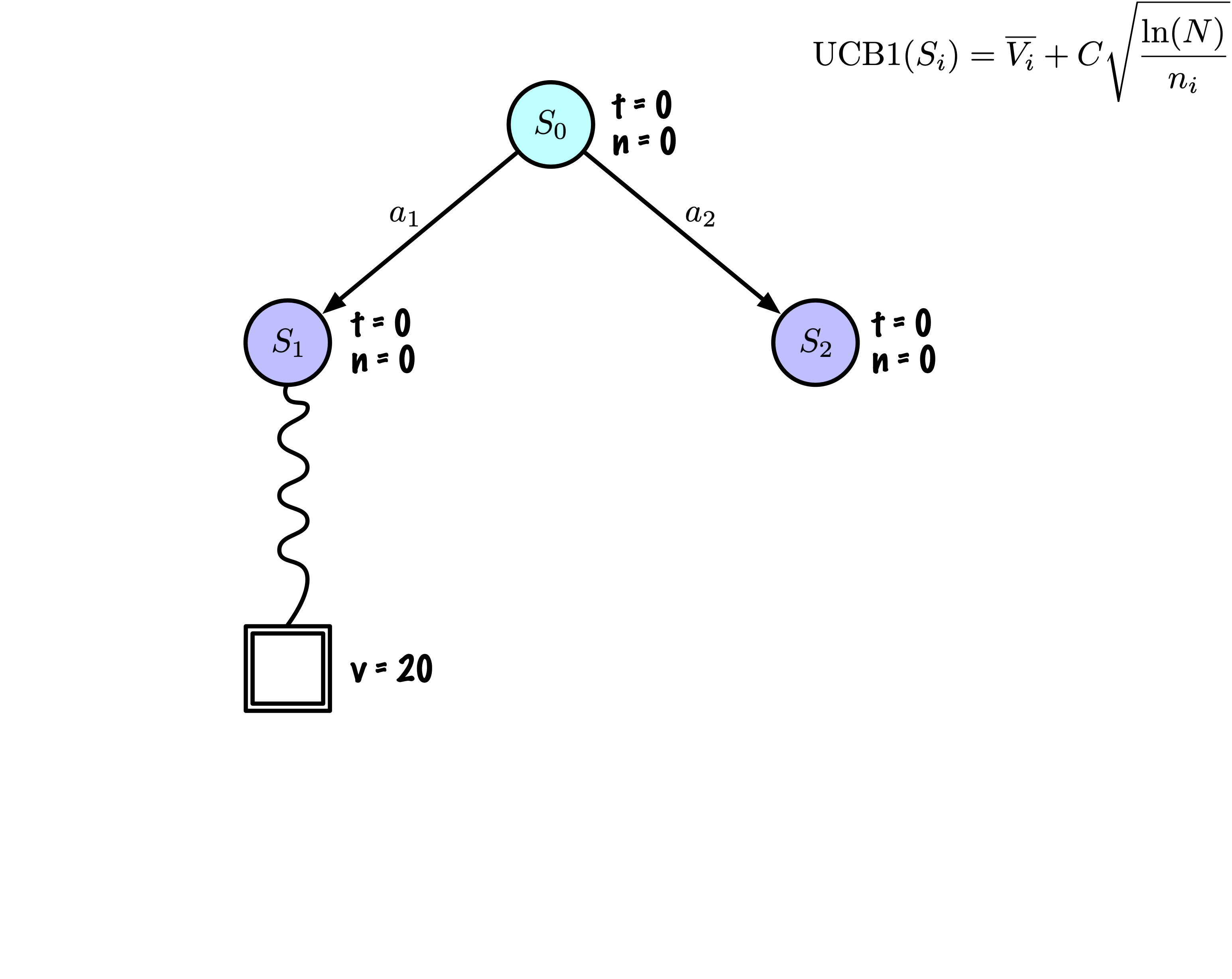
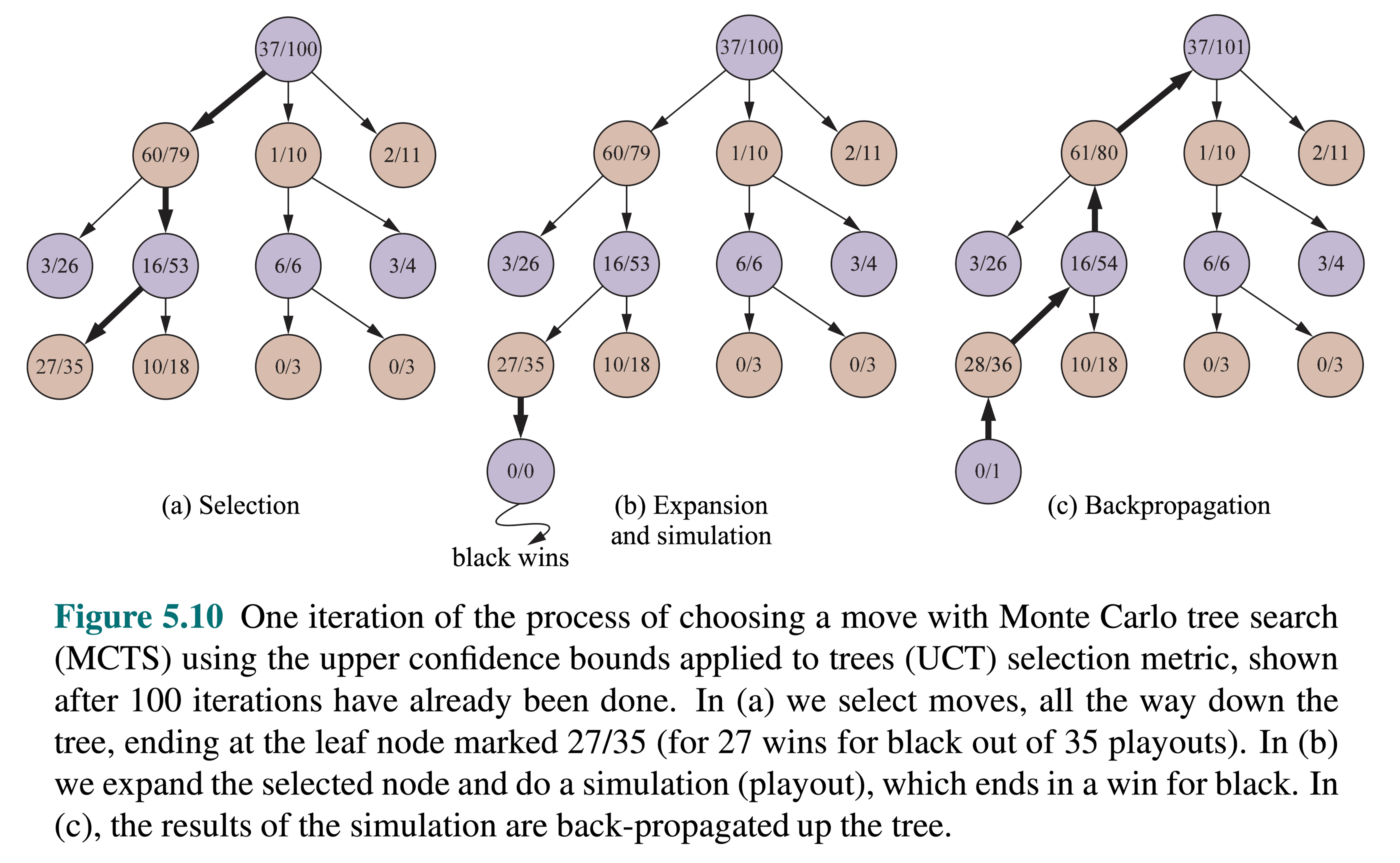
Russell and Norvig
Summary: tree building
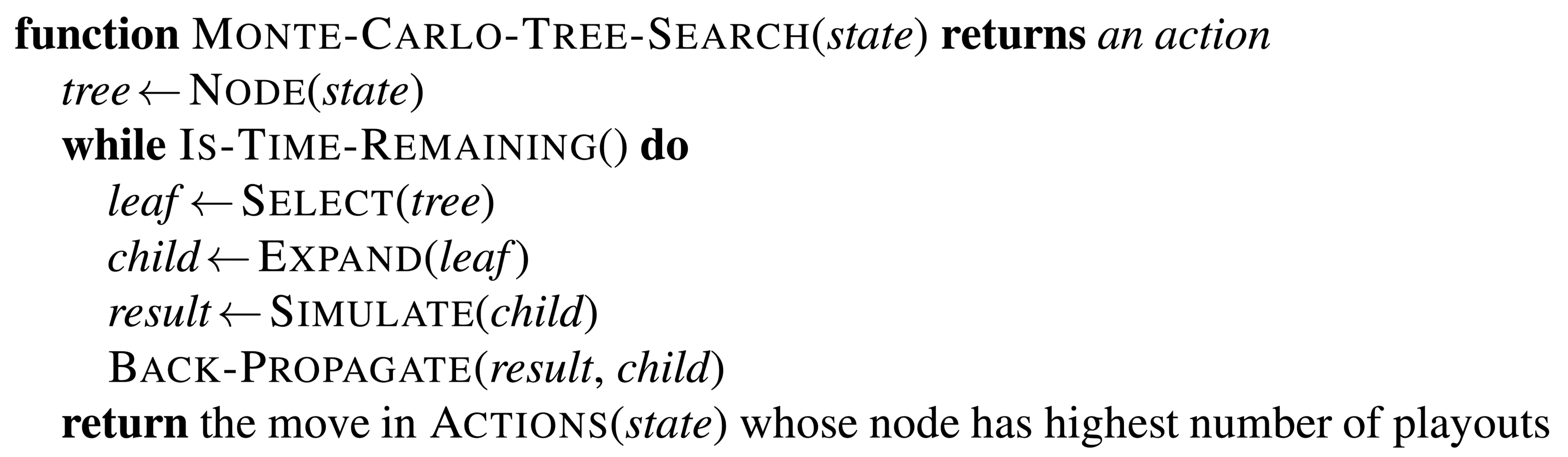
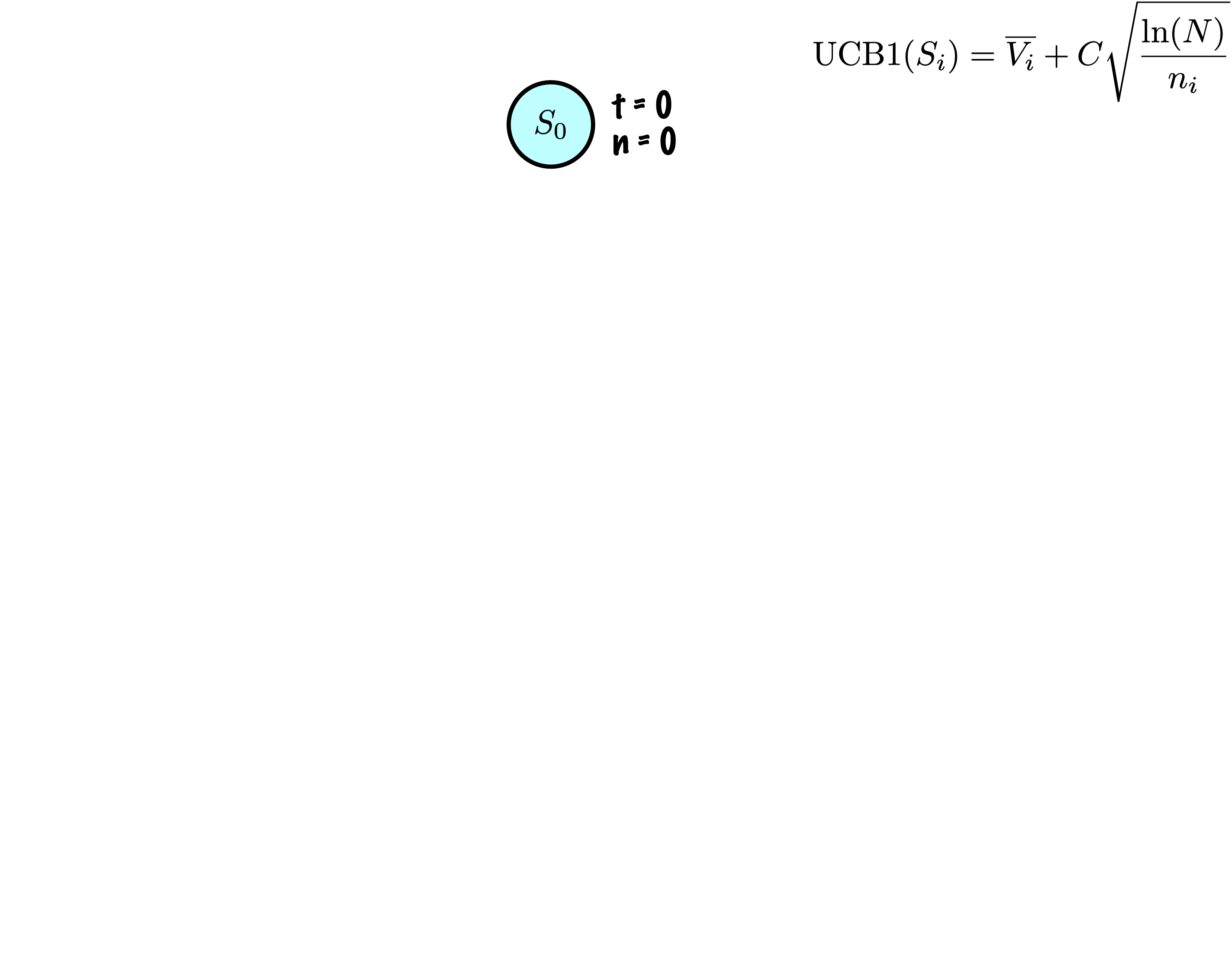
Initially, the tree has one node, it is \(S_0\).
We add its descendants and we are ready to start.
The Monte Carlo Tree Search slowly builds its search tree.
Summary: 4 steps
With each iteration, the following steps occur:
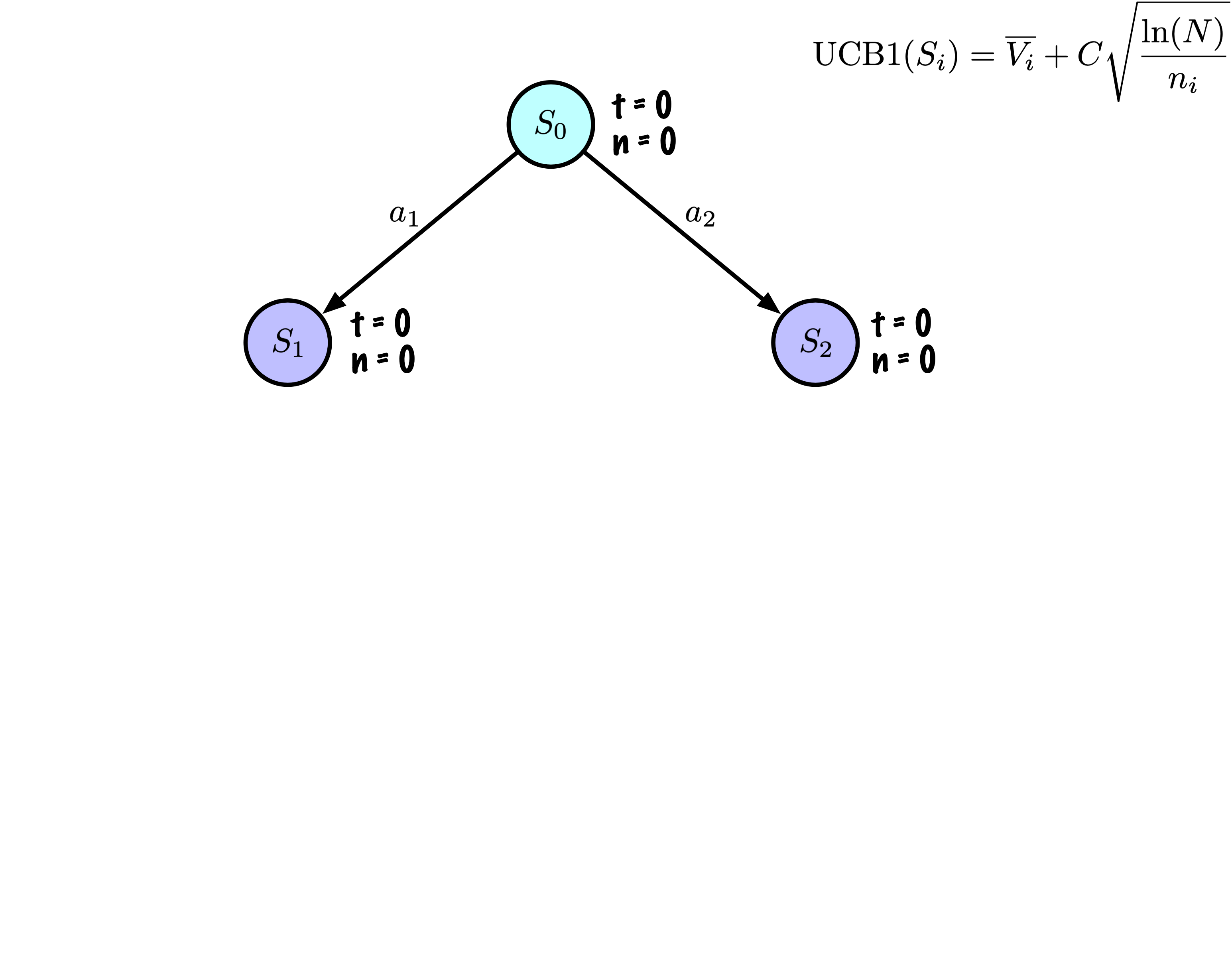
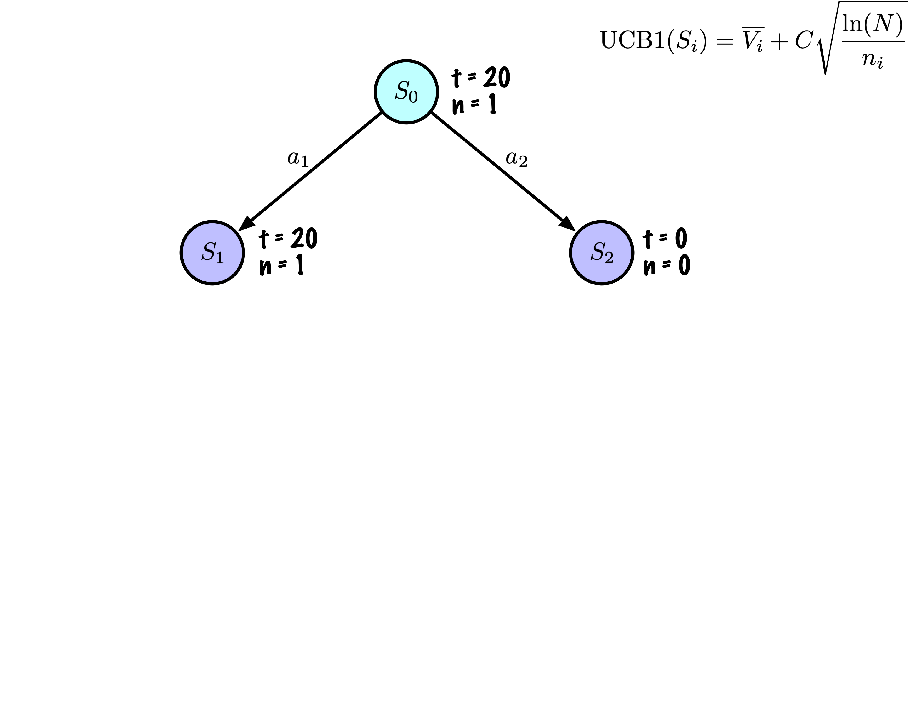
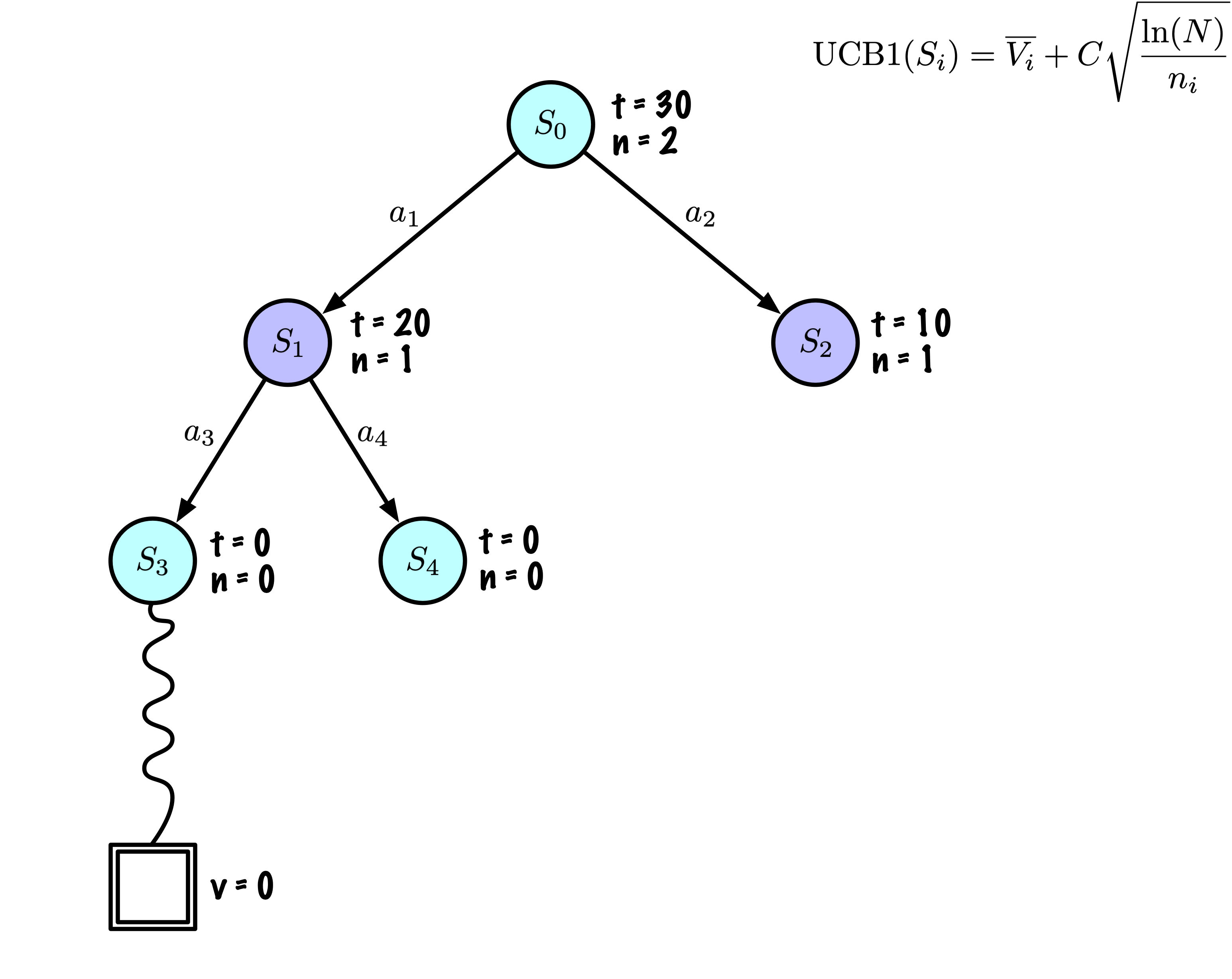
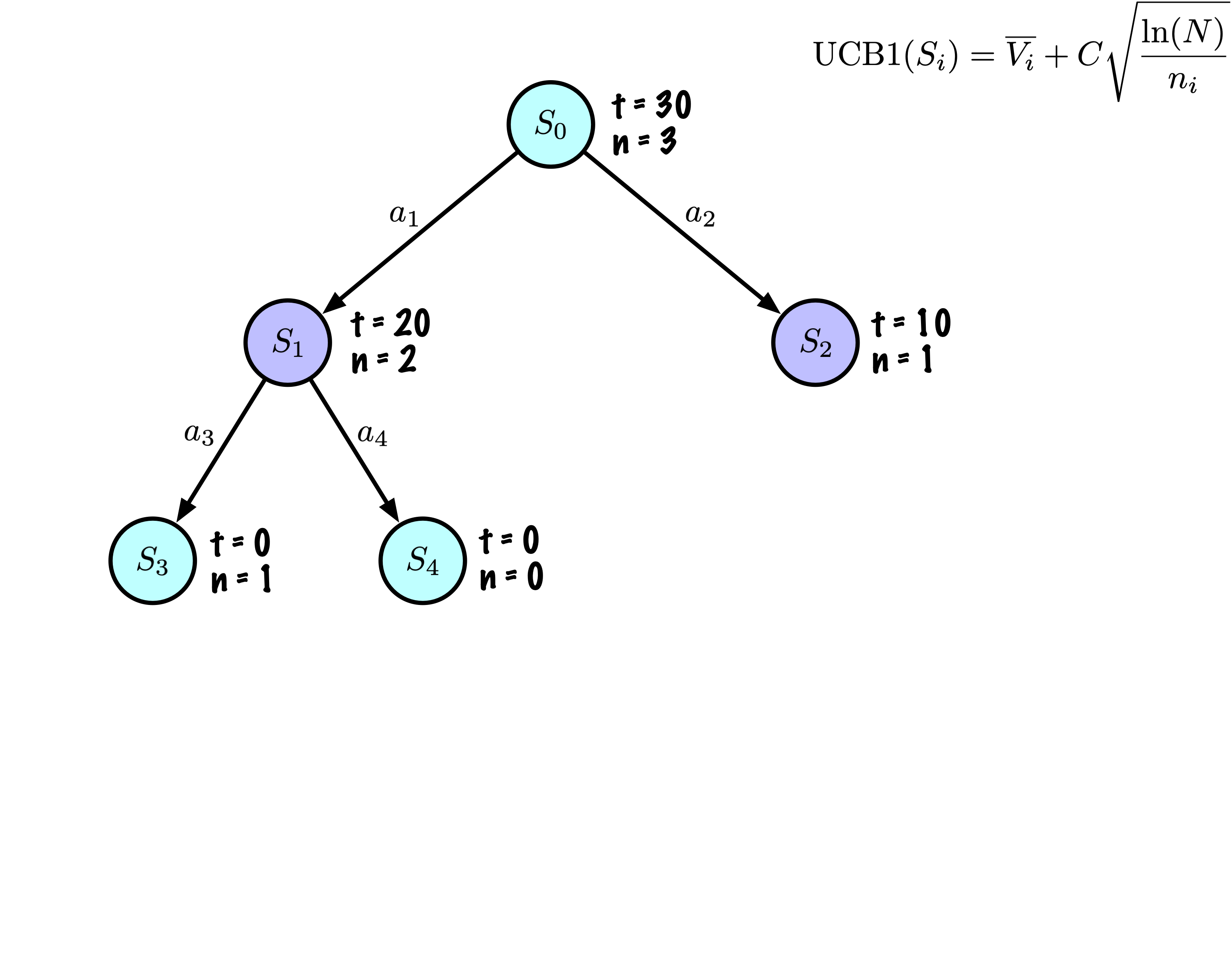
Selection: Identify the “best” node by descending a single path in the tree, guided by UCB1.
Expansion: Expand the node if it is a leaf in the MCTS Tree and \(n \gt 0\).
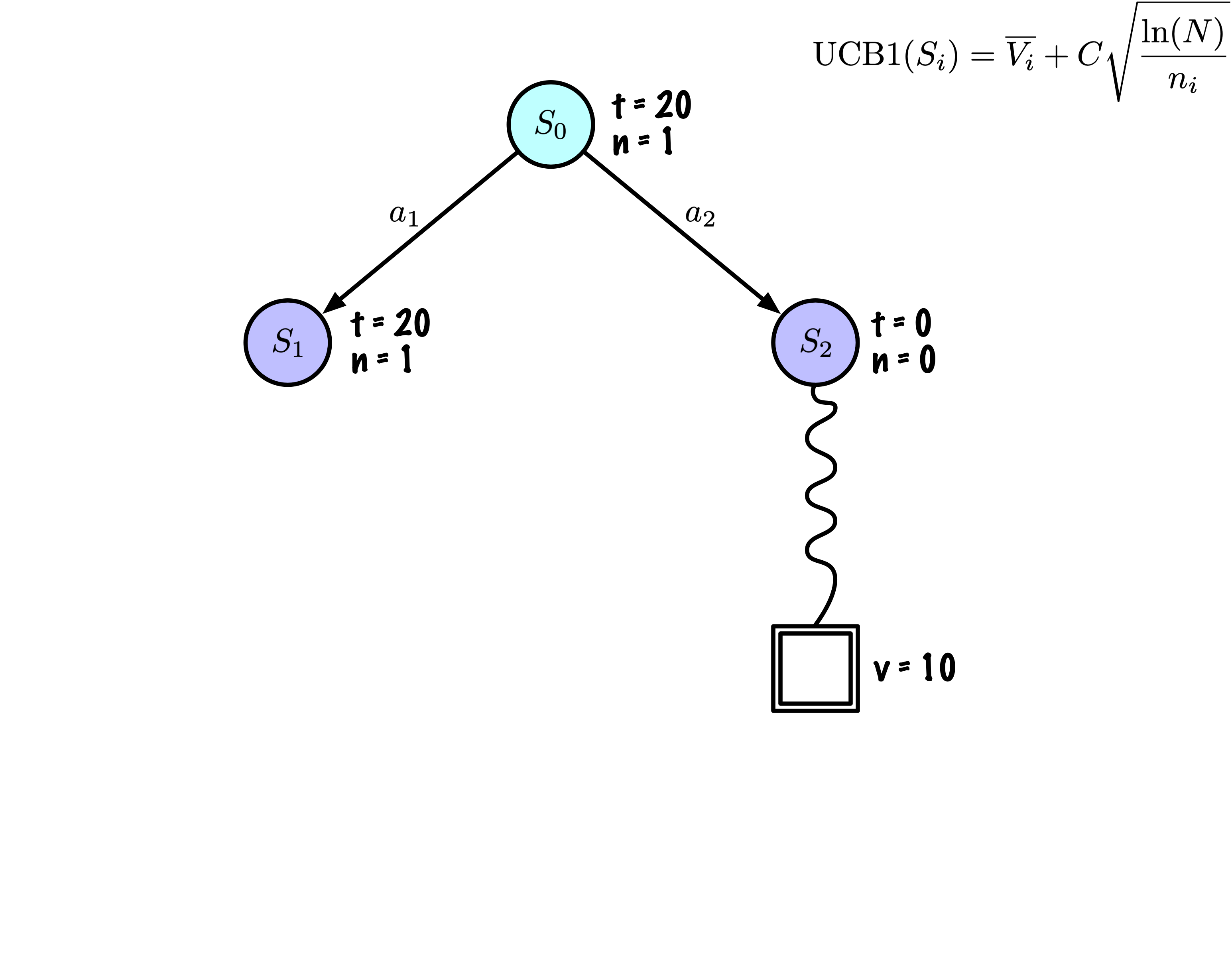
Rollout: Simulate a game from the current state to a terminal state by randomly selecting actions.
Backpropagation: Use the obtained information to update the current node and all parent nodes up to the root.
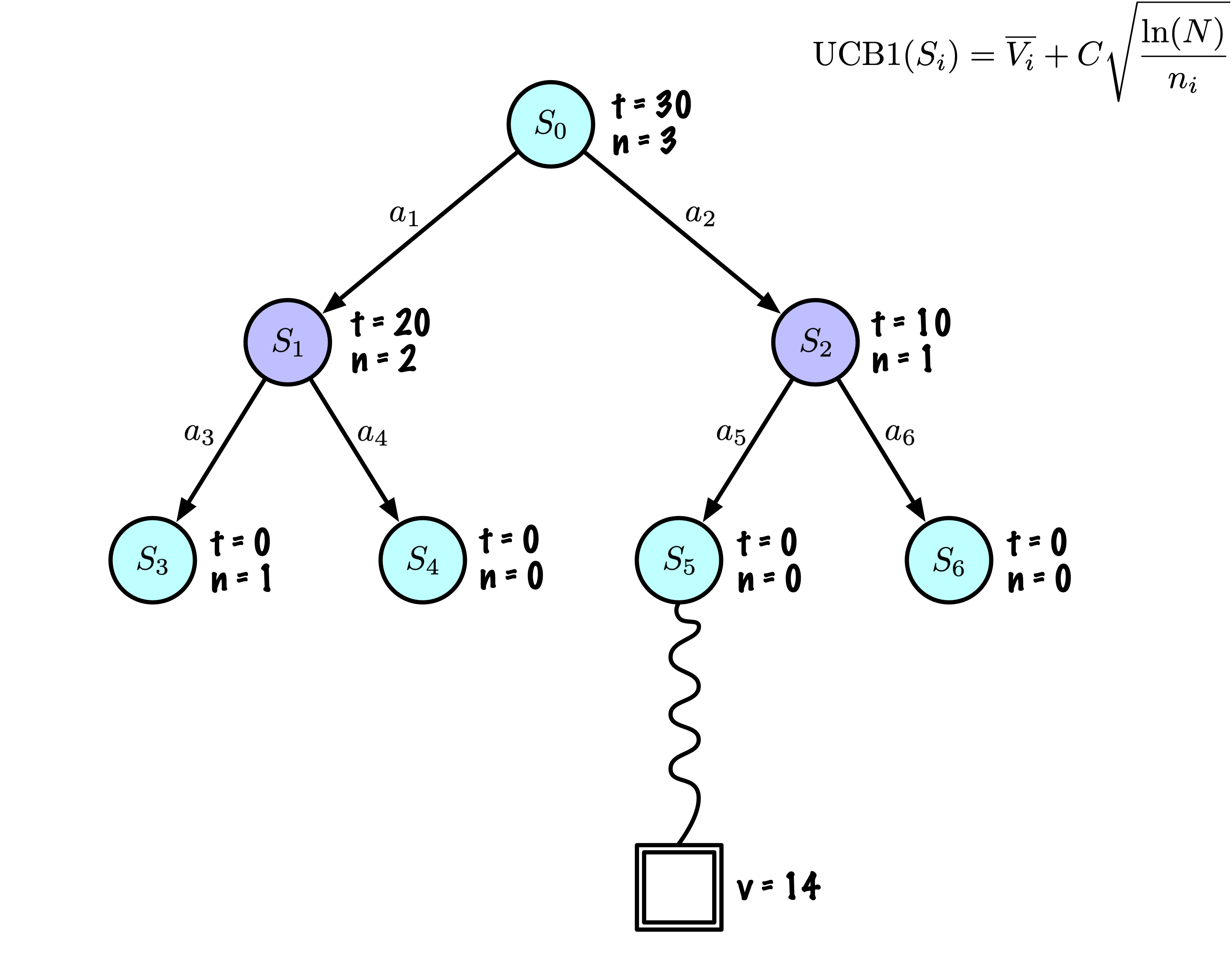
Summary: nodes
Each node records its total score and visit count.
This information is used to calculate a value that guides tree descent, balancing exploration and exploitation.
Summary: exploration vs exploitation
\[
\mathrm{UCB1}(S_i) = \overline{V_i} + C \sqrt{\frac{\ln(N)}{n_i}}
\]
The usual value for \(C\) is \(\sqrt{2}\).
Exploration essentially occurs when two nodes have approximately the same average score, then MCTS favours nodes with fewer visits (dividing by \(n\)).
For \(n \lt \ln(N)\), the value of the ratio is greater than 1, whereas for \(n \gt \ln(N)\), the ratio becomes less than 1.
So there is a small fraction of the time where exploration kicks in. But even then, the contribution of the ratio is quite tame, we’re taking the square root of that ratio, multiplied by \(\sqrt{2} \sim 1.414213562\).
Summary: exploration vs exploitation
In simulated annealing, the initial temperature and the scale of the objective function are linked.
Acceptance rule for a candidate move with score change \(\Delta E = E_{\text{new}} - E_{\text{old}}\):
If \(\Delta E \le 0\): always accept (better or equal solution).
If \(\Delta E > 0\): accept with probability
\[
p = \exp(-\Delta E / T).
\]
Summary: exploration vs exploitation
In Simulated Annealing:
\(T\) defines how “big” a bad move has to be before it is unlikely to be accepted.
If \(T\) is large compared to typical \(\Delta E\):
Even sizeable worsening moves have reasonable probability.
Very exploratory.
If \(T\) is small:
Only very small worsening moves are accepted.
Mostly exploitative / hill-climbing.
That’s why you often pick initial \(T\) using the distribution of \(\Delta E\) on random states: e.g., “set \(T_0\) so that a typical \(\Delta E\) has, say, 60-80% acceptance.” It’s explicitly tied to the scale of the scoring function.
Summary: C as an exploration scale
In UCT (UCB1) we’re using
\[
\text{score}(i)
= V_i + C \sqrt{\frac{\ln N}{n_i}},
\]
where:
\(V_i\): average playout value of child \(i\) (exploitation term),
\(N\): total visits to the parent node,
\(n_i\): visits to child \(i\),
\(C\): exploration constant.
Summary: C as an exploration scale
At a given node:
The child with largest \(\text{score}(i)\) is selected.
The second term \[
C \sqrt{\frac{\ln N}{n_i}}
\] is pure exploration: large when \(n_i\) is small, shrinking as you visit that child.
Summary: C as an exploration scale
Consider two children, 1 and 2. You choose 2 instead of 1 when:
The difference in average playout values that can be “overruled” by exploration is proportional to \(C\).
Larger\(C\) → exploration term dominates more → you’re willing to try a child whose \(V_i\) is significantly worse, just because it’s under-explored.
Smaller\(C\) → you stick more to the currently best-looking\(V_i\).
Summary: C as an exploration scale
In the classical UCB1 theory, rewards are assumed to be in \([0,1]\), and there’s a specific recommended constant (e.g. \(\sqrt{2}\)). If your reward scale is different (say in \([-1,1]\) or large magnitude), you essentially rescale that constant; in practice people tune \(C\) empirically.
Summary: C as an exploration scale
Analogy:
Simulated annealing’s \(T\) and MCTS’s \(C\) both balance exploration vs exploitation.
In both cases, their effective meaning depends on the scale of the objective / rewards.
In SA: “how bad can a move be and still often be accepted?”
In MCTS: “how much worse can a child’s current \(V_i\) be and still get chosen for exploration?”
Summary: C as an exploration scale
Key differences:
Simulated Annealing:
Single trajectory.
\(T\) is explicitly scheduled (high to low) over time.
Balances local moves in a single search path.
Summary: C as an exploration scale
MCTS (UCT):
Tree of many paths.
\(C\) is constant, but exploration decays automatically via \(\sqrt{\ln N / n_i}\):
Early: \(n_i\) small → high exploration.
Late: \(n_i\) big → exploration term shrinks, behavior gets more greedy.
Core Game Framework
Game
Code
import mathimport randomimport numpy as npimport matplotlib.pyplot as pltclass Game:""" Abstract interface for a deterministic, 2-player, zero-sum, turn-taking game. Conventions (used by Tic-Tac-Toe and the solvers below): - Players are identified by strings "X" and "O". - evaluate(state) returns: > 0 if the position is good for "X" < 0 if the position is good for "O" == 0 for a draw or non-terminal equal position """def initial_state(self):"""Return an object representing the starting position of the game."""raiseNotImplementedErrordef get_valid_moves(self, state):""" Given a state, return an iterable of legal moves. The type of 'move' is game-dependent (e.g., (row, col) for Tic-Tac-Toe). """raiseNotImplementedErrordef make_move(self, state, move, player):""" Return the successor state obtained by applying 'move' for 'player' to 'state'. The original state should not be modified in-place. """raiseNotImplementedErrordef get_opponent(self, player):"""Return the opponent of 'player'."""raiseNotImplementedErrordef is_terminal(self, state):""" Return True if 'state' is a terminal position (win, loss, or draw), False otherwise. """raiseNotImplementedErrordef evaluate(self, state):""" Return a scalar evaluation of 'state': +1 for X win, -1 for O win, 0 otherwise (for Tic-Tac-Toe). For other games this may be generalized, but here we keep it simple. """raiseNotImplementedErrordef display(self, state):"""Print a human-readable representation of 'state' (for debugging)."""raiseNotImplementedError
TicTacToe
Code
class TicTacToe(Game):""" Classic 3x3 Tic-Tac-Toe implementation using a NumPy array of strings. Empty squares are represented by " ". Player "X" is assumed to be the maximizing player. """def__init__(self):self.size =3def initial_state(self):"""Return an empty 3x3 board."""return np.full((self.size, self.size), " ")def get_valid_moves(self, state):"""All (i, j) pairs where the board cell is empty."""return [ (i, j)for i inrange(self.size)for j inrange(self.size)if state[i, j] ==" " ]def make_move(self, state, move, player):""" Return a new board with 'player' placed at 'move' (row, col). The original state is not modified. """ new_state = state.copy() new_state[move] = playerreturn new_statedef get_opponent(self, player):"""Swap player labels between 'X' and 'O'."""return"O"if player =="X"else"X"def is_terminal(self, state):""" A state is terminal if: - Either player has a 3-in-a-row (evaluate != 0), or - There are no empty squares left (draw). """ifself.evaluate(state) !=0:returnTruereturn" "notin statedef evaluate(self, state):""" Return +1 if X has three in a row, -1 if O has three in a row, and 0 otherwise (including non-terminal states and draws). This is a "game-theoretic" evaluation at terminal states; for non-terminal positions we simply return 0. """ lines = []# Rows and columnsfor i inrange(self.size): lines.append(state[i, :]) # row i lines.append(state[:, i]) # column i# Main diagonals lines.append(np.diag(state)) lines.append(np.diag(np.fliplr(state)))# Check each line for a winfor line in lines:if np.all(line =="X"):return1if np.all(line =="O"):return-1return0def display(self, state):""" Visualize a Tic-Tac-Toe board using matplotlib. Parameters ---------- state : np.ndarray of shape (size, size) Board containing ' ', 'X', or 'O'. """ size =self.size fig, ax = plt.subplots() ax.set_aspect('equal') ax.set_xlim(0, size) ax.set_ylim(0, size)# Draw grid linesfor i inrange(1, size): ax.axhline(i, color='black') ax.axvline(i, color='black')# Hide axes completely ax.axis('off')# Draw X and O symbolsfor i inrange(size):for j inrange(size): cx = j +0.5 cy = size - i -0.5# invert y-axis for correct row orientation symbol = state[i, j]if symbol =="X": ax.plot(cx, cy, marker='x', markersize=40* (3/size), color='blue', markeredgewidth=3)elif symbol =="O": circle = plt.Circle((cx, cy), radius=0.30* (3/size), fill=False, color='red', linewidth=3) ax.add_patch(circle) plt.show()
Solver
Code
class Solver:""" Base class for all solvers (Random, Minimax, AlphaBeta, MCTS, etc.). Solvers must implement: - select_move(game, state, player) Solvers may optionally implement: - reset() : called at the start of each game - opponent_played() : used by persistent solvers (e.g., MCTS) Notes ----- • Solvers may keep internal state that persists across moves. • GameRunner may call reset() automatically before every match. """def select_move(self, game, state, player):""" Must be implemented by subclasses. Returns a legal move for the given player. """raiseNotImplementedErrordef get_name(self):""" Return the solver's name for reporting, logging, or tournament results. The default returns the class name, but solvers may override to include parameters (e.g., "MCTS(num_simulations=500)""). """returnself.__class__.__name__def opponent_played(self, move):""" Optional. Called after the opponent moves. Useful for stateful solvers like MCTS. Stateless solvers can ignore it. """passdef reset(self):""" Optional. Called once at the beginning of each game. Override only if the solver maintains internal state (e.g., MCTS tree, cached analysis, heuristic tables). """pass
RandomSolver
Code
class RandomSolver(Solver):""" A simple baseline solver: - At each move, chooses uniformly at random among all legal moves. - Does not maintain any internal state (no learning). """def__init__(self, seed=None):self.rng = random.Random(seed)def select_move(self, game, state, player):"""Return a random legal move for the current player.""" moves = game.get_valid_moves(state)returnself.rng.choice(moves)def opponent_played(self, move):"""Random solver has no internal state to update."""pass
GameRunner
Code
class GameRunner:""" Utility to run a single game between two solvers on a given Game. This class is deliberately simple: it alternates moves between "X" and "O" until a terminal state is reached. """def__init__(self, game, verbose=False):self.game = gameself.verbose = verbosedef play_game(self, solver_X, solver_O):""" Play one full game: - solver_X controls player "X" - solver_O controls player "O" Returns ------- result : int +1 if X wins, -1 if O wins, 0 for a draw. """ state =self.game.initial_state() player ="X" solvers = {"X": solver_X, "O": solver_O}# Play until terminal positionwhilenotself.game.is_terminal(state):# Current player selects a move move = solvers[player].select_move(self.game, state, player)# Apply the move state =self.game.make_move(state, move, player)ifself.verbose:self.game.display(state)# Notify the opponent (for persistent solvers like MCTS) opp =self.game.get_opponent(player) solvers[opp].opponent_played(move)# Switch active player player = oppifself.verbose:print(self.game.evaluate(state), "\n")# Final evaluation from X's perspectivereturnself.game.evaluate(state)
evaluate_solvers
Code
def evaluate_solvers(game, solver_X, solver_O, num_games, verbose=False):""" Evaluate two solvers head-to-head on a given game. Parameters ---------- game : Game An instance of a Game (e.g., TicTacToe). solver_X : Solver Solver controlling player "X" (the maximizing player). solver_O : Solver Solver controlling player "O" (the minimizing player). num_games : int Number of games to play with these fixed roles. Notes ----- - The same solver instances are reused across games. This allows *persistent* solvers (e.g., MCTS) to accumulate experience across games. - Outcomes are interpreted from X's perspective: +1 -> X wins -1 -> O wins 0 -> draw """ runner = GameRunner(game)# Aggregate statistics over all games results = {"X_wins": 0,"O_wins": 0,"draws": 0, }for i inrange(num_games):# Play one game with solver_X as "X" and solver_O as "O" outcome = runner.play_game(solver_X, solver_O)# Update counters based on outcome (+1, -1, or 0)if outcome ==1: results["X_wins"] +=1if verbose:print(f"Game {i +1}: X wins") elif outcome ==-1: results["O_wins"] +=1if verbose:print(f"Game {i +1}: O wins") else: results["draws"] +=1if verbose:print(f"Game {i +1}: Draw")# Print final summaryif verbose:print(f"\nAfter {num_games} games:")print(f" X ({solver_X.get_name()}) wins: {results['X_wins']}")print(f" O ({solver_O.get_name()}) wins: {results['O_wins']}")print(f" Draws: {results['draws']}")return results
MinimaxSolver
Code
from functools import lru_cachedef canonical(state):""" Convert a NumPy array board into a hashable, immutable representation (tuple of tuples). This allows us to use it as a key in dicts or as an argument to lru_cache. MCTS can also reuse this representation. """returntuple(map(tuple, state))class MinimaxSolver(Solver):""" A classic, exact Minimax solver for Tic-Tac-Toe. - Assumes "X" is the maximizing player. - Uses memoization (lru_cache) to avoid recomputing values for identical positions. """def select_move(self, game, state, player):""" Public interface: choose the best move for 'player' using Minimax. For Tic-Tac-Toe we can safely search the full game tree. """# Store game on self so _minimax can use itself.game = game# From X's perspective: X is maximizing, O is minimizing maximizing = (player =="X")# For Tic-Tac-Toe, depth=9 is enough to cover all remaining moves. _, move =self._minimax(canonical(state), player, maximizing, 9)return move@lru_cache(maxsize=None)def _minimax(self, state_key, player, maximizing, depth):""" Internal recursive minimax. Parameters ---------- state_key : hashable representation of the board (tuple of tuples) player : player to move at this node ("X" or "O") maximizing: True if this node is a 'max' node (X to move), False if this is a 'min' node (O to move) depth : remaining search depth (not used for cutoffs in this full-search Tic-Tac-Toe implementation, but kept for didactic purposes and easy extension). """# Recover the NumPy board from the canonical state_key state = np.array(state_key)# Terminal test: win, loss, or drawifself.game.is_terminal(state):# Evaluation is always from X's perspective: +1, -1, or 0returnself.game.evaluate(state), None moves =self.game.get_valid_moves(state) best_move =Noneif maximizing:# X to move: maximize the evaluation best_val =-math.inffor move in moves: st2 =self.game.make_move(state, move, player) val, _ =self._minimax( canonical(st2),self.game.get_opponent(player),False, depth -1 )if val > best_val: best_val = val best_move = movereturn best_val, best_moveelse:# O to move: minimize the evaluation (since evaluation is for X) best_val = math.inffor move in moves: st2 =self.game.make_move(state, move, player) val, _ =self._minimax( canonical(st2),self.game.get_opponent(player),True, depth -1 )if val < best_val: best_val = val best_move = movereturn best_val, best_move
MinimaxAlphaBetaSolver
Code
class MinimaxAlphaBetaSolver(Solver):""" A classical Minimax solver enhanced with Alpha-Beta pruning. - Assumes "X" is the maximizing player. - Uses memoization (lru_cache) to avoid recomputing states. - Performs a *full* search of Tic-Tac-Toe (depth=9). - Returns the optimal move for the current player. """# ------------------------------------------------------------# Solver interface# ------------------------------------------------------------def select_move(self, game, state, player):""" Public interface required by Solver. Runs Alpha-Beta search from the current state. """self.game = game maximizing = (player =="X") # X maximizes, O minimizes# Reset cache between games to avoid storing millions of keysself._alphabeta.cache_clear() value, move =self._alphabeta( canonical(state), player, maximizing,9, # full-depth search-math.inf, # alpha math.inf # beta )return move# ------------------------------------------------------------# Internal alpha-beta with memoization# ------------------------------------------------------------@lru_cache(maxsize=None)def _alphabeta(self, state_key, player, maximizing, depth, alpha, beta):""" Parameters ---------- state_key : tuple-of-tuples board player : player whose turn it is ('X' or 'O') maximizing: True if this node is a maximizing node for X depth : remaining depth alpha : best guaranteed value for maximizer so far beta : best guaranteed value for minimizer so far """ state = np.array(state_key)# Terminal or horizon caseifself.game.is_terminal(state) or depth ==0:returnself.game.evaluate(state), None moves =self.game.get_valid_moves(state) best_move =None# --------------------------------------------------------# MAX (X)# --------------------------------------------------------if maximizing: value =-math.inffor move in moves: st2 =self.game.make_move(state, move, player) child_val, _ =self._alphabeta( canonical(st2),self.game.get_opponent(player),False, # now minimizing depth -1, alpha, beta )if child_val > value: value = child_val best_move = move alpha =max(alpha, value)if beta <= alpha:break# β-cutoffreturn value, best_move# --------------------------------------------------------# MIN (O)# --------------------------------------------------------else: value = math.inffor move in moves: st2 =self.game.make_move(state, move, player) child_val, _ =self._alphabeta( canonical(st2),self.game.get_opponent(player),True, # now maximizing depth -1, alpha, beta )if child_val < value: value = child_val best_move = move beta =min(beta, value)if beta <= alpha:break# α-cutoffreturn value, best_move
Sanity Check
game = TicTacToe()a = RandomSolver(7)b = MinimaxSolver()results = evaluate_solvers(game, a, b, num_games=100)results
{'X_wins': 0, 'O_wins': 82, 'draws': 18}
Sanity Check
game = TicTacToe()a = RandomSolver(7)b = MinimaxAlphaBetaSolver()results = evaluate_solvers(game, a, b, num_games=100)results
{'X_wins': 0, 'O_wins': 82, 'draws': 18}
Implementation
MCTSClassicSolver
Code
class MCTSClassicSolver(Solver):""" A textbook, first-contact implementation of Monte Carlo Tree Search (MCTS) for deterministic 2-player zero-sum games (e.g., Tic-Tac-Toe). Key ideas: - For each decision, we build a tree rooted at the current position. - Each node stores: * state: board position * player: player to move in this state ("X" or "O") * N: visit count * W: total reward from this node player's perspective * children: move -> child Node * untried_moves: list of legal moves not yet expanded * parent: link to the parent node (for backpropagation) - One MCTS *simulation* = selection → expansion → simulation (rollout) → backpropagation. - We throw away the tree after returning a move (no learning). """class Node:"""A single node in the MCTS search tree."""def__init__(self, state, player, parent=None, moves=None):self.state = state # board position (NumPy array)self.player = player # player to move in this stateself.parent = parent # parent Node (None for root)self.children = {} # move -> child Nodeself.untried_moves =list(moves) if moves isnotNoneelse []self.N =0# visit countself.W =0.0# total reward (this player's perspective)def__init__(self, num_simulations=500, exploration_c=math.sqrt(2), seed=None):""" Parameters ---------- num_simulations : int Number of simulations (playouts) to run per move. exploration_c : float Exploration constant C in the UCT formula. seed : int or None Optional random seed for reproducibility. """self.num_simulations = num_simulationsself.exploration_c = exploration_cself.rng = random.Random(seed)self.game =Noneself.root =None# root Node for the current search# ------------------------------------------------------------# Public Solver interface# ------------------------------------------------------------def select_move(self, game, state, player):""" Choose a move for 'player' in 'state' using classic MCTS. A new tree is built from scratch for this call. The tree is not reused for later moves or games. """self.game = gameself.root =None# root Node for the current search# Create the root node for the current position. root_state = state.copy() root_moves =self.game.get_valid_moves(root_state)self.root =self.Node(root_state, player, parent=None, moves=root_moves)# Run multiple simulations starting from the root.for _ inrange(self.num_simulations):self._run_simulation()# After simulations, choose the child with the largest visit count.ifnotself.root.children:# No children: no legal moves (terminal). Fall back to random if needed. moves =self.game.get_valid_moves(self.root.state)returnself.rng.choice(moves) if moves elseNone best_move =None best_visits =-1for move, child inself.root.children.items():if child.N > best_visits: best_visits = child.N best_move = movereturn best_movedef opponent_played(self, move):""" Classic MCTS here is stateless across moves and games: we rebuild the tree for every decision. So we do not need to track the opponent's move. """pass# ------------------------------------------------------------# Internal MCTS steps# ------------------------------------------------------------def _run_simulation(self):""" Perform one MCTS simulation from the root. 1. Selection: descend the tree using UCT until we reach a node that is terminal or has untried moves. 2. Expansion: if the node is non-terminal and has untried moves, expand one child. 3. Simulation (rollout): from the new child, play random moves to the end of the game. 4. Backpropagation: update N and W along the path with the outcome. """ node =self.root# 1. SELECTION: descend while fully expanded and non-terminal.whileTrue:ifself.game.is_terminal(node.state):# Terminal position: evaluate immediately. outcome =self.game.evaluate(node.state) # from X's perspectiveself._backpropagate(node, outcome)returnif node.untried_moves:# 2. EXPANSION: choose one untried move and create a child node. move =self.rng.choice(node.untried_moves) node.untried_moves.remove(move) next_state =self.game.make_move(node.state, move, node.player) next_player =self.game.get_opponent(node.player) next_moves =self.game.get_valid_moves(next_state) child =self.Node(next_state, next_player, parent=node, moves=next_moves) node.children[move] = child# 3. SIMULATION: rollout from the newly created child. outcome =self._rollout(child.state, child.player)# 4. BACKPROPAGATION: update all nodes on the path from child to root.self._backpropagate(child, outcome)return# Node is fully expanded and non-terminal → choose a child by UCT. node =self._select_child(node)def _select_child(self, node):""" UCT selection: for each child V_parent(child) = - (child.W / child.N) UCT = V_parent(child) + C * sqrt( ln(N_parent + 1) / N_child ) We store W and N from the child's own perspective, so we negate child.W / child.N to get the parent's perspective. """ parent_visits = node.N best_score =-math.inf best_child =Nonefor move, child in node.children.items():if child.N ==0: score = math.inf # always explore unvisited children at least onceelse:# Average reward from the child's own perspective. avg_child = child.W / child.N# Parent and child players alternate; reward from parent perspective# is the negative of the child's perspective. reward_parent =-avg_child exploration =self.exploration_c * math.sqrt( math.log(parent_visits +1) / child.N ) score = reward_parent + explorationif score > best_score: best_score = score best_child = childreturn best_childdef _rollout(self, state, player_to_move):""" Random playout from 'state' until the game ends. Returns the final result from X's perspective: +1 if X wins, -1 if O wins, 0 for draw. """ current_state = state.copy() current_player = player_to_movewhilenotself.game.is_terminal(current_state): moves =self.game.get_valid_moves(current_state) move =self.rng.choice(moves) current_state =self.game.make_move(current_state, move, current_player) current_player =self.game.get_opponent(current_player)returnself.game.evaluate(current_state)def _backpropagate(self, node, outcome):""" Backpropagate the simulation outcome up the tree. outcome is always from X's perspective: +1, -1, or 0. For each node on the path from 'node' up to the root: - Convert outcome to that node's player's perspective: reward = outcome if node.player == "X" = -outcome if node.player == "O" - Update: node.N += 1 node.W += reward """ current = nodewhile current isnotNone:if current.player =="X": reward = outcomeelse: reward =-outcome current.N +=1 current.W += reward current = current.parent
Node
class MCTSClassicSolver(Solver):class Node:def__init__(self, state, player, parent=None, moves=None):self.state = state # board position (NumPy array)self.player = player # player to move in this stateself.parent = parent # parent Node (None for root)self.children = {} # move -> child Nodeself.untried_moves =list(moves) if moves isnotNoneelse []self.N =0# visit countself.W =0.0# total reward (this player's perspective)
def select_move(self, game, state, player):self.game = gameself.root =None# building a new tree for each call# Create the root node for the current position. root_state = state.copy() root_moves =self.game.get_valid_moves(root_state)self.root =self.Node(root_state, player, parent=None, moves=root_moves)# Run multiple simulations starting from the root.for _ inrange(self.num_simulations):self._run_simulation() best_move =None best_visits =-1for move, child inself.root.children.items():if child.N > best_visits: best_visits = child.N best_move = movereturn best_move
Public Solver interface
def opponent_played(self, move):pass
_run_simulation
def _run_simulation(self): node =self.root# 1. SELECTION: descend while fully expanded and non-terminal.whileTrue:ifself.game.is_terminal(node.state):# Terminal position: evaluate immediately. outcome =self.game.evaluate(node.state) # from X's perspectiveself._backpropagate(node, outcome)returnif node.untried_moves:# 2. EXPANSION: choose one untried move and create a child node. move =self.rng.choice(node.untried_moves) node.untried_moves.remove(move) next_state =self.game.make_move(node.state, move, node.player) next_player =self.game.get_opponent(node.player) next_moves =self.game.get_valid_moves(next_state) child =self.Node(next_state, next_player, parent=node, moves=next_moves) node.children[move] = child# 3. SIMULATION: rollout from the newly created child. outcome =self._rollout(child.state, child.player)# 4. BACKPROPAGATION: update all nodes on the path from child to root.self._backpropagate(child, outcome)return# Node is fully expanded and non-terminal → choose a child by UCT. node =self._select_child(node)
_select_child
def _select_child(self, node): parent_visits = node.N best_score =-math.inf best_child =Nonefor move, child in node.children.items():if child.N ==0: score = math.inf # always explore unvisited children at least onceelse:# Average reward from the child's own perspective. avg_child = child.W / child.N# Parent and child players alternate; reward from parent perspective# is the negative of the child's perspective. reward_parent =-avg_child exploration =self.exploration_c * math.sqrt( math.log(parent_visits +1) / child.N ) score = reward_parent + explorationif score > best_score: best_score = score best_child = childreturn best_child
def _backpropagate(self, node, outcome): current = nodewhile current isnotNone:if current.player =="X": reward = outcomeelse: reward =-outcome current.N +=1 current.W += reward current = current.parent
visualize_tree
Code
from graphviz import Digraphdef visualize_tree(root, max_depth=3, show_mcts_stats=True, show_edge_labels=True):""" Visualize a game tree rooted at `root` using Graphviz. Assumes: - `root` is a Node with attributes: state, player, children: dict[move -> Node], N, W. - This matches the Node used in MCTSClassicSolver. Parameters ---------- root : Node Root of the (sub)tree to visualize. max_depth : int Maximum depth to recurse (root at depth 0). show_mcts_stats : bool If True, include N and V for each node (compact vertical layout). show_edge_labels : bool If True, label edges with the move (e.g., (row, col)). """ dot = Digraph(format="png") dot.edge_attr.update( fontsize="8", fontname="Comic Sans MS" )# Make the tree compact dot.graph_attr.update( rankdir="TB", # top-to-bottom nodesep="0.15", # horizontal spacing ranksep="0.50", # vertical spacing ) dot.node_attr.update( shape="box", fontsize="9", fontname="Comic Sans MS", margin="0.02,0.02", )def add_node(node, node_id, depth):if depth > max_depth:return# Build compact labelif show_mcts_stats and node.N >0: V = node.W / node.N# player on top, then N, then V (vertical) label =f"{node.player}\\nN={node.N}\\nV={V:.2f}"else: label =f"{node.player}" dot.node(node_id, label=label)# Recurse on childrenif depth == max_depth:returnfor move, child in node.children.items(): child_id =f"{id(child)}"if show_edge_labels: dot.edge(node_id, child_id, label=str(move))else: dot.edge(node_id, child_id) add_node(child, child_id, depth +1) add_node(root, "root", depth=0)return dot
def tally_scores(game):""" Enumerate all complete games of Tic-Tac-Toe from the initial position (X to move) and tally how many end in: - X win - draw - O win Returns ------- overall : dict {'X': total_X_wins, 'draw': total_draws, 'O': total_O_wins} table : list[list[dict]] A 3x3 list of dicts. For each cell (i, j), table[i][j] = {'X': ..., 'draw': ..., 'O': ...} counts games where X's *first move* was at (i, j). """ size = game.size # should be 3 for standard Tic-Tac-Toe# Overall tallies for all games overall = {'X': 0, 'draw': 0, 'O': 0}# Per-first-move tallies as a 3x3 grid table = [ [ {'X': 0, 'draw': 0, 'O': 0} for _ inrange(size) ]for _ inrange(size) ]def recurse(state, player, first_move):""" Depth-first enumeration of all complete games. Parameters ---------- state : board position (NumPy array) player : 'X' or 'O' (player to move) first_move : None, or (row, col) of X's very first move """# Base case: terminal state → classify outcomeif game.is_terminal(state): v = game.evaluate(state) # +1 (X win), -1 (O win), 0 (draw)if v >0: outcome ='X'elif v <0: outcome ='O'else: outcome ='draw'# Update overall tally overall[outcome] +=1# If we know X's first move, update that cell's tally tooif first_move isnotNone: i, j = first_move table[i][j][outcome] +=1return# Recursive case: expand all legal movesfor move in game.get_valid_moves(state): next_state = game.make_move(state, move, player) next_player = game.get_opponent(player)# Record X's very first moveif first_move isNoneand player =="X": fm = move # this becomes the first_move for the rest of this branchelse: fm = first_move recurse(next_state, next_player, fm)# Start from the empty board, X to move, and no first_move yet initial_state = game.initial_state() recurse(initial_state, player="X", first_move=None)return overall, tabledef print_tally_table(table):""" Print a 3x3 table of tallies. Each cell shows: X:<wins> D:<draws> O:<wins> where counts are restricted to games where X's first move was played in that cell. """ size =len(table)for i inrange(size): row_cells = []for j inrange(size): stats = table[i][j] cell_str =f"X:{stats['X']} D:{stats['draw']} O:{stats['O']}" row_cells.append(cell_str)print(" | ".join(row_cells))print()def print_tally_table_percentages(table):""" Print a 3x3 table of tallies. Each cell shows: X:<wins> D:<draws> O:<wins> where counts are restricted to games where X's first move was played in that cell. """ size =len(table)for i inrange(size): row_cells = []for j inrange(size): stats = table[i][j] cell_str =f"X:{stats['X']/255168:.2%} D:{stats['draw']/255168:.2%} O:{stats['O']/255168:.2%}" row_cells.append(cell_str)print(" | ".join(row_cells))print()game = TicTacToe()overall, table = tally_scores(game)print("Overall tally:")print(overall) # {'X': ..., 'draw': ..., 'O': ...}print("\nTallies by X's first move (3x3 grid):")print_tally_table(table)print("\nTallies by X's first move (3x3 grid) as percentages:")print_tally_table_percentages(table)
Overall tally:
{‘X’: 131184, ‘draw’: 46080, ‘O’: 77904}
{‘X’: 51.41%, ‘draw’: 18.06%, ‘O’: 30.53%}
Tallies by X’s first move (3x3 grid, X/draw/O):
14652/5184/7896
14232/5184/10176
14652/5184/7896
14232/5184/10176
15648/4608/5616
14232/5184/10176
14652/5184/7896
14232/5184/10176
14652/5184/7896
Tallies by X’s first move (3x3 grid, X/draw/O) as percentages:
5.74% / 2.03% / 3.09%
5.58% / 2.03% / 3.99%
5.74% / 2.03% / 3.09%
5.58% / 2.03% / 3.99%
6.13% / 1.81% / 2.20%
5.58% / 2.03% / 3.99%
5.74% / 2.03% / 3.09%
5.58% / 2.03% / 3.99%
5.74% / 2.03% / 3.09%
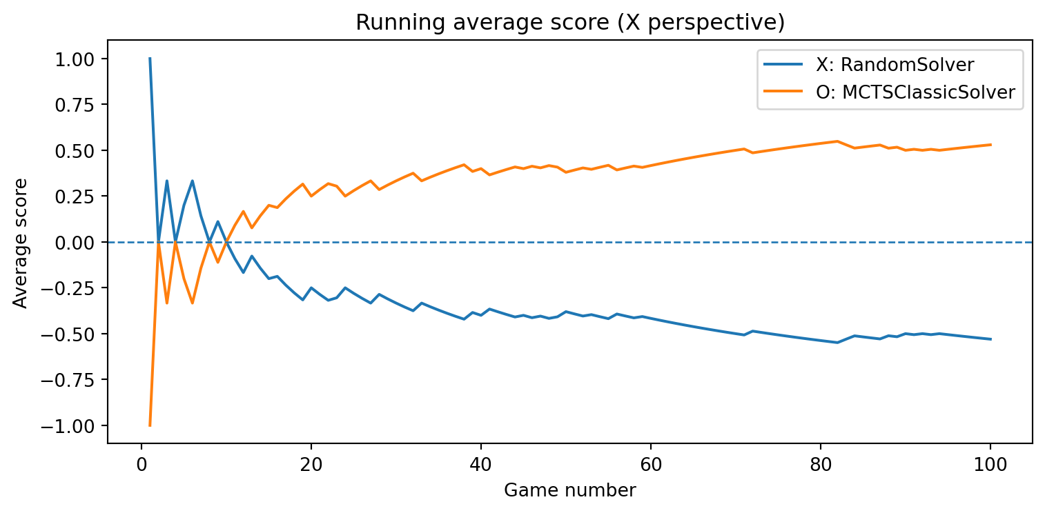
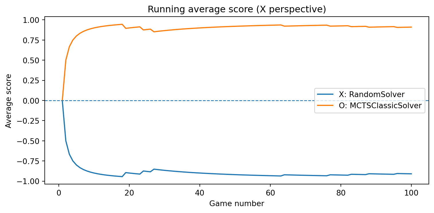
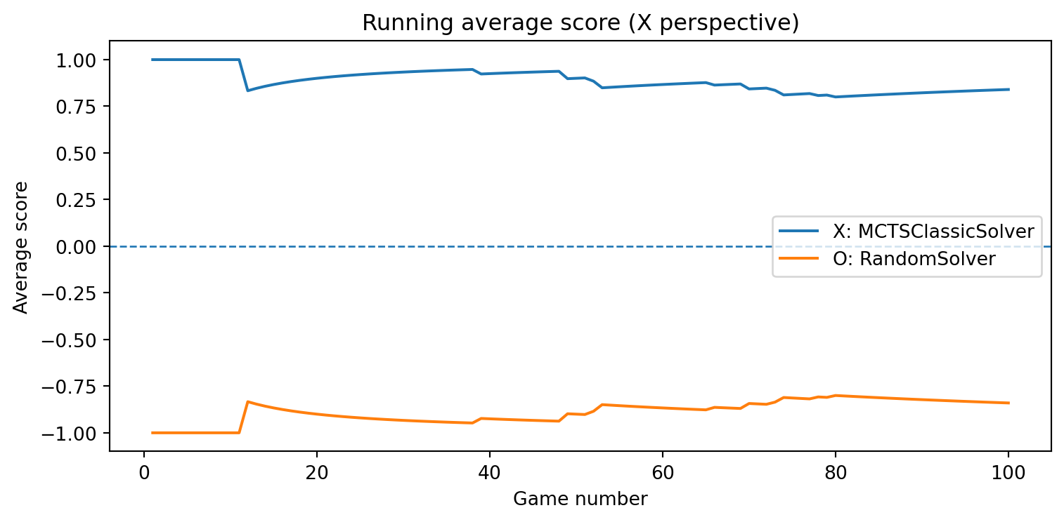
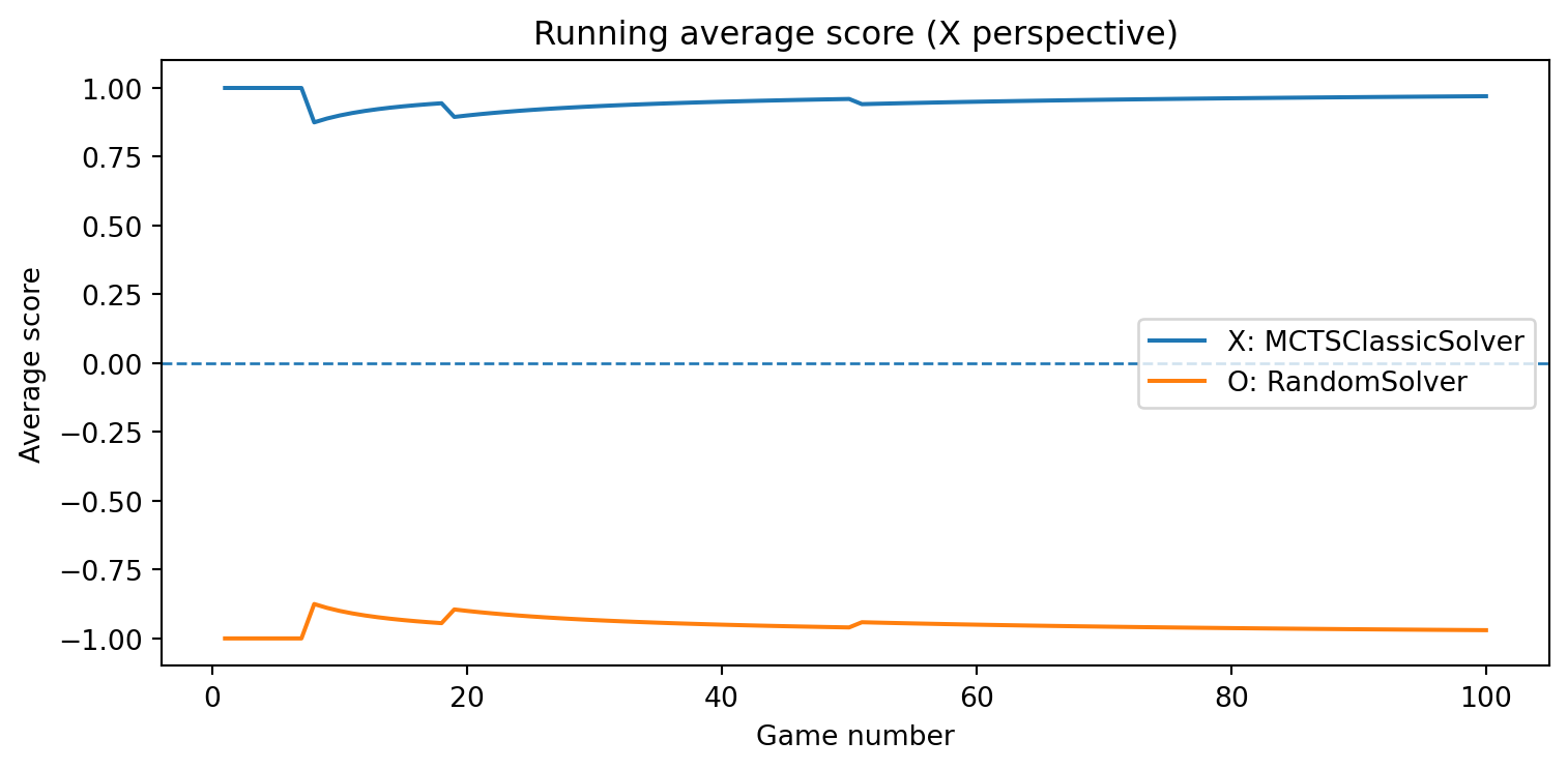
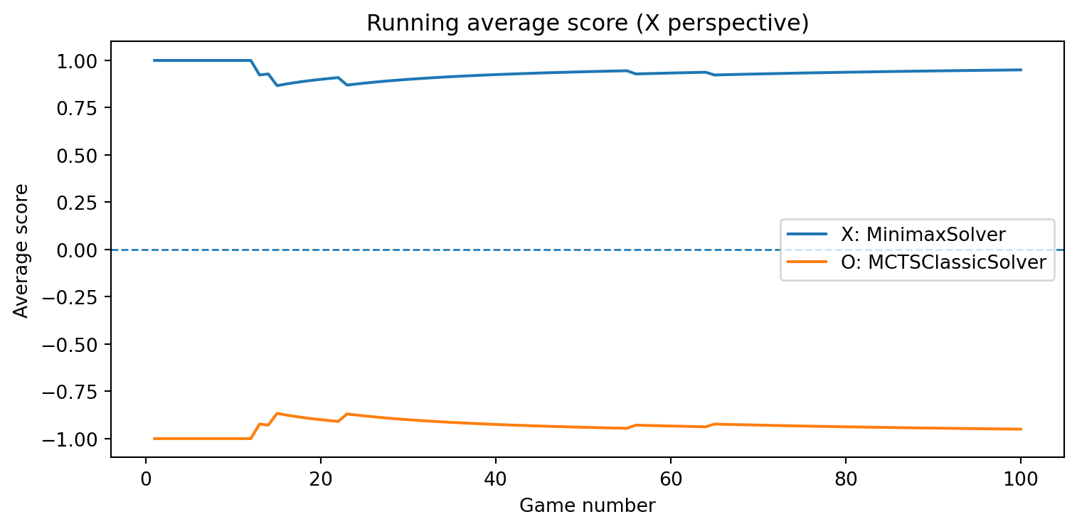
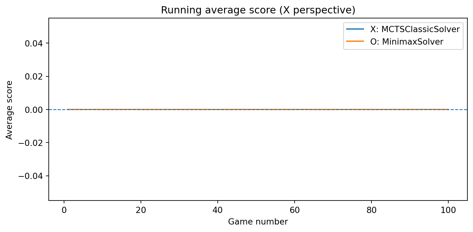
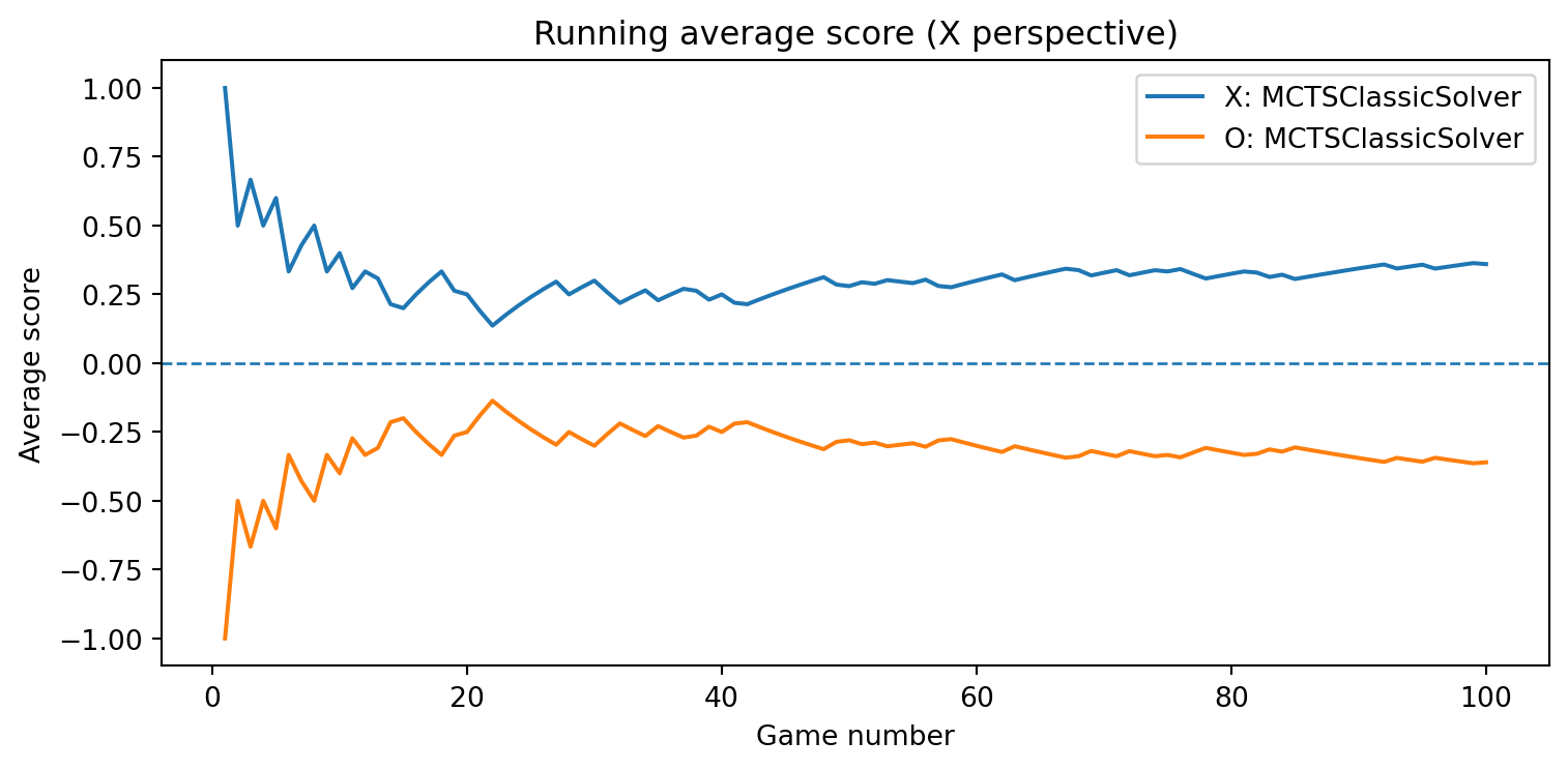
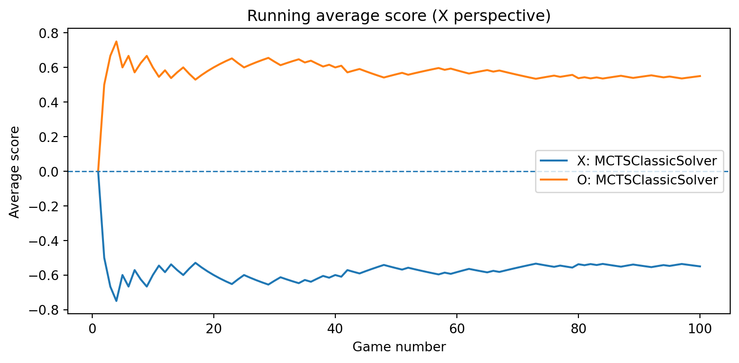
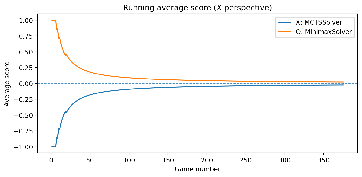
evaluate_solvers_with_plot
Code
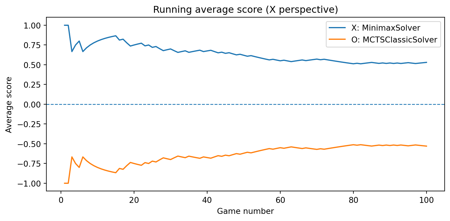
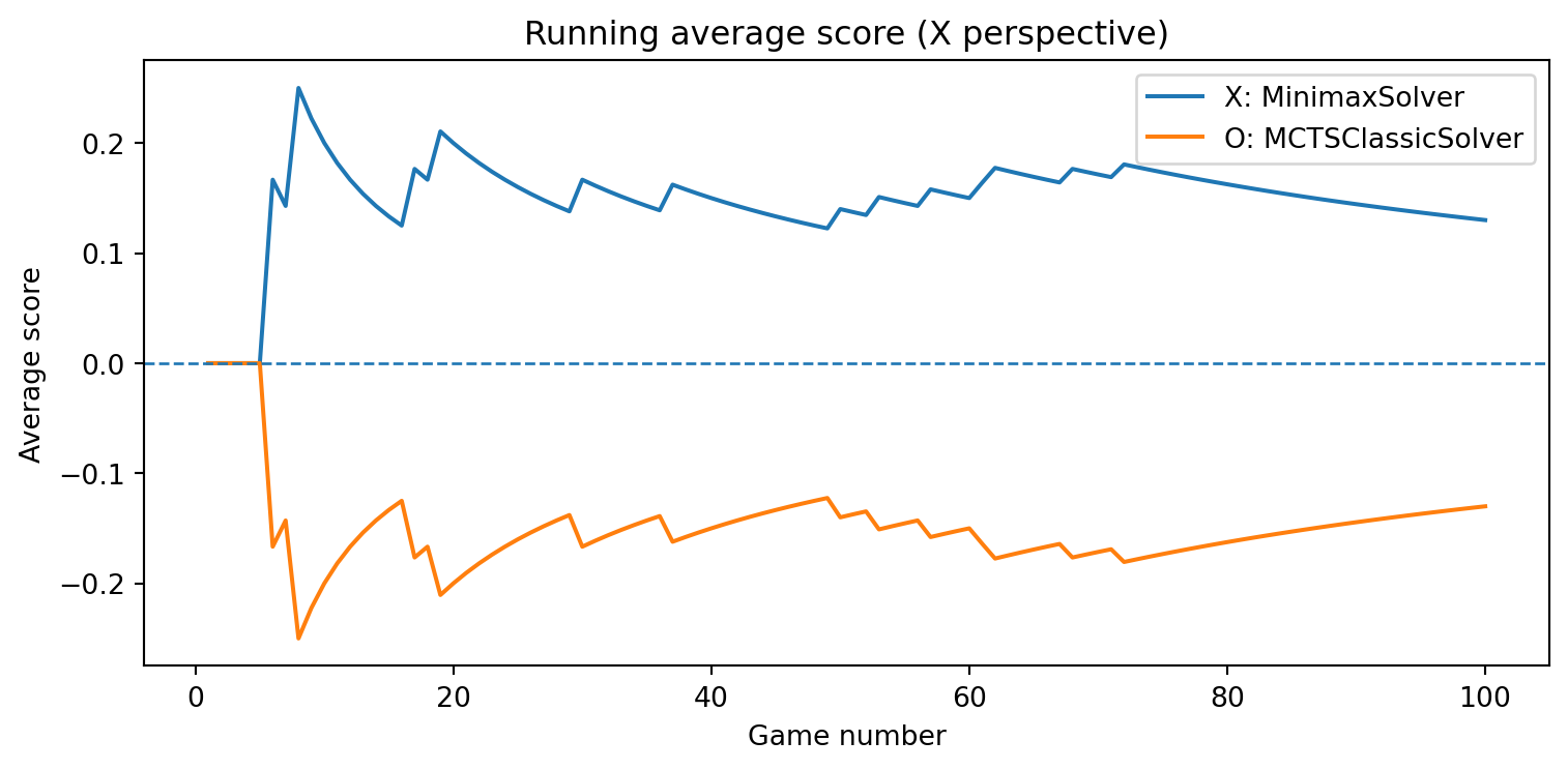
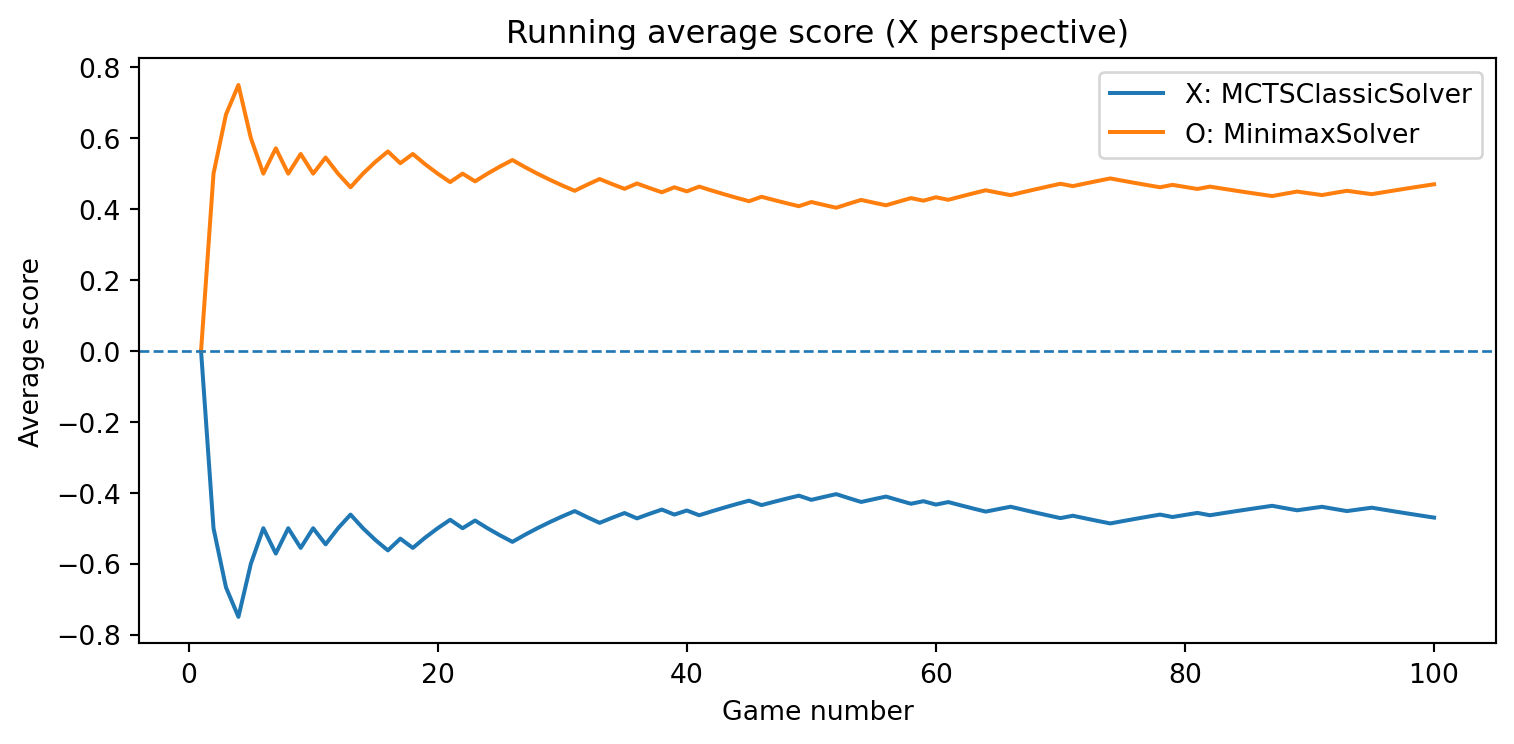
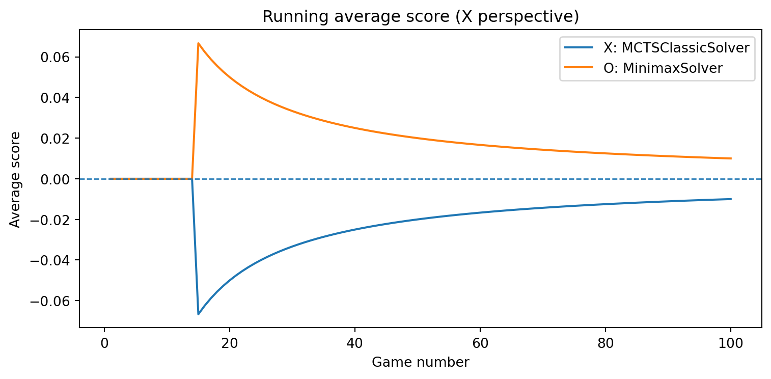
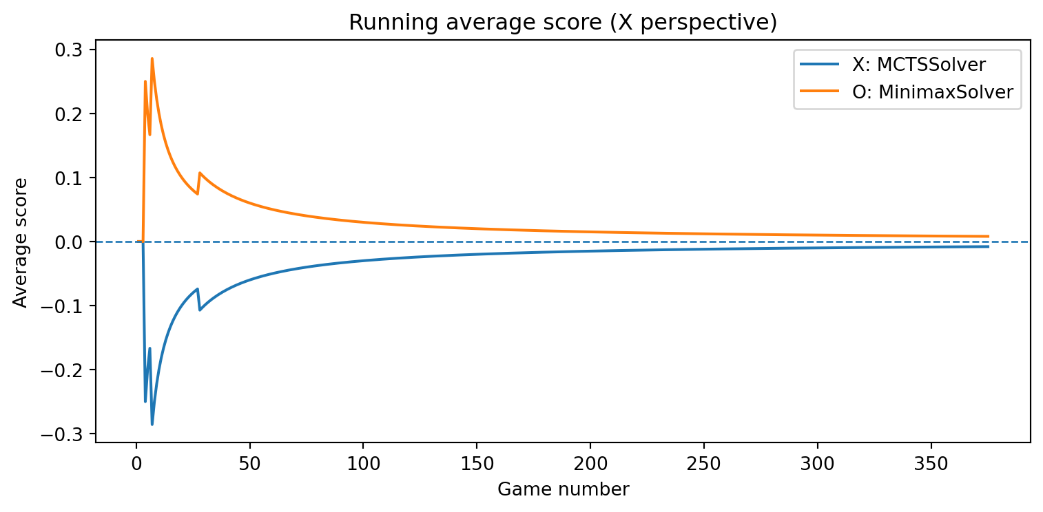
def evaluate_solvers_with_plot(game, solver_X, solver_O, num_games):""" Play 'num_games' games between solver_X (as 'X') and solver_O (as 'O'), track cumulative performance, and plot running average scores. Scoring is from X's perspective: outcome = +1 if X wins outcome = -1 if O wins outcome = 0 if draw The running average score for O is simply the negative of X's running average (zero-sum). """ runner = GameRunner(game)# Counters for final summary results = {"X_wins": 0,"O_wins": 0,"draws": 0, }# For plotting: running average score as a function of game index avg_scores_X = [] avg_scores_O = [] cumulative_score_X =0.0for i inrange(num_games): outcome = runner.play_game(solver_X, solver_O)# Update win/draw countersif outcome ==1: results["X_wins"] +=1elif outcome ==-1: results["O_wins"] +=1else: results["draws"] +=1# Update cumulative score (from X's perspective) cumulative_score_X += outcome avg_X = cumulative_score_X / (i +1) avg_O =-avg_X # zero-sum avg_scores_X.append(avg_X) avg_scores_O.append(avg_O)# Plot running average scores games =range(1, num_games +1) plt.figure(figsize=(8, 4)) plt.plot(games, avg_scores_X, label=f"X: {solver_X.get_name()}") plt.plot(games, avg_scores_O, label=f"O: {solver_O.get_name()}") plt.axhline(0.0, linestyle="--", linewidth=1) plt.xlabel("Game number") plt.ylabel("Average score") plt.title("Running average score (X perspective)") plt.legend() plt.tight_layout() plt.show()return results, avg_scores_X, avg_scores_O
class MCTSSolver(Solver):""" Monte Carlo Tree Search solver for deterministic, zero-sum, two-player games like Tic-Tac-Toe. Key ideas: - The solver maintains a search tree keyed by canonical(state). - Each node stores: * N: visit count * W: total reward from the perspective of the player to move at that node (positive is good for that player) * children: mapping move -> child_state_key * untried_moves: moves that have not been expanded yet * player: the player to move at this node ("X" or "O") - select_move(): * Ensures the current state is in the tree. * Runs a fixed number of simulations from the current root. * Returns the move leading to the most visited child. - opponent_played(move): * Advances the internal root along the actual move played (if that move has been explored). * This allows the solver to reuse search statistics across moves and across games. """def__init__(self, num_simulations=500, exploration_c=math.sqrt(2), seed=None):""" Parameters ---------- num_simulations : int Number of MCTS simulations to run per move. exploration_c : float Exploration constant 'c' in the UCT formula. seed : int or None Optional random seed for reproducibility. """self.num_simulations = num_simulationsself.exploration_c = exploration_cself.rng = random.Random(seed)# The search tree: state_key -> node dictionaryself.tree = {}# Current root in the treeself.root_key =None# canonical(state)self.root_player =None# player to move at the root ("X" or "O")# Game reference (set on first select_move)self.game =None# -----------------------------# Public API# -----------------------------def select_move(self, game, state, player):""" Choose a move for 'player' from 'state' using Monte Carlo Tree Search. This method: 1. Synchronizes the internal root with the provided state. 2. Runs a fixed number of MCTS simulations from the root. 3. Returns the move leading to the child with the largest visit count. """self.game = game state_key = canonical(state)# Ensure the root in the tree corresponds to the current state.# If this state has been seen before, we reuse its node and statistics.self.root_key = state_keyself.root_player = playerself._get_or_create_node(state_key, player)# Run MCTS simulations starting from the current rootfor _ inrange(self.num_simulations):self._run_simulation()# After simulations, pick the child with the highest visit count. root_node =self.tree[self.root_key]ifnot root_node["children"]:# No children: must be a terminal state or no legal moves.# Fall back to any valid move (or raise error); here we pick at random. moves =self.game.get_valid_moves(np.array(self.root_key))returnself.rng.choice(moves) best_move =None best_visits =-1for move, child_key in root_node["children"].items(): child =self.tree[child_key]if child["N"] > best_visits: best_visits = child["N"] best_move = movereturn best_movedef opponent_played(self, move):""" Update the internal root based on the opponent's move. This is called by GameRunner after the other player has made a move. We try to move the root to the corresponding child node: - If the move was explored, we reuse that subtree. - Otherwise, we create a fresh node for the resulting state. """# If we do not yet have a root or a game reference, nothing to do.ifself.root_key isNoneorself.game isNone:return root_node =self.tree.get(self.root_key)if root_node isNone:# Should not happen, but be robust.self.root_key =Noneself.root_player =Nonereturn# If we already explored this move from the root, just move down the tree.if move in root_node["children"]: child_key = root_node["children"][move]self.root_key = child_keyself.root_player =self.tree[child_key]["player"]return# Otherwise, we need to apply the move on the board and create a new node. state = np.array(self.root_key) player_who_played = root_node["player"] next_state =self.game.make_move(state, move, player_who_played) next_key = canonical(next_state) next_player =self.game.get_opponent(player_who_played)self.root_key = next_keyself.root_player = next_playerself._get_or_create_node(next_key, next_player)# -----------------------------# Internal helpers# -----------------------------def _get_or_create_node(self, state_key, player_to_move):""" Ensure that a node for 'state_key' exists in the tree. If not present, create it with: - N = 0, W = 0 - untried_moves = all valid moves from this state - children = {} - player = player_to_move """if state_key notinself.tree: state = np.array(state_key)self.tree[state_key] = {"N": 0, # visit count"W": 0.0, # total reward from this node's player's perspective"children": {}, # move -> child_state_key"untried_moves": self.game.get_valid_moves(state),"player": player_to_move, }returnself.tree[state_key]def _run_simulation(self):""" Perform one MCTS simulation from the current root: 1. SELECTION: Follow the tree using UCT until we reach a node with untried_moves or a terminal state. 2. EXPANSION: If the node has untried_moves and is non-terminal, expand one move. 3. ROLLOUT: From the new leaf, play random moves to a terminal state. 4. BACKPROPAGATION: Propagate the final outcome back along the visited path. """ifself.root_key isNone:return# nothing to do state_key =self.root_key state = np.array(state_key) path = [] # list of state_keys visited along this simulation# -------------------------# 1–2. Selection & Expansion# -------------------------whileTrue: path.append(state_key) node =self.tree[state_key]# If this is a terminal state, stop and evaluate directly.ifself.game.is_terminal(state): outcome =self.game.evaluate(state) # from X's perspectivebreak# If there are untried moves, expand one of them.if node["untried_moves"]: move = node["untried_moves"].pop() next_state =self.game.make_move(state, move, node["player"]) next_key = canonical(next_state) next_player =self.game.get_opponent(node["player"])# Create the child node if it does not yet exist.self._get_or_create_node(next_key, next_player)# Link child in the tree node["children"][move] = next_key# The rollout starts from this new leaf node. state_key = next_key state = next_state path.append(state_key) outcome =self._rollout(state, next_player)break# Otherwise, the node is fully expanded: select a child using UCT. move, child_key =self._select_child(node) state_key = child_key state = np.array(state_key)# -------------------------# 4. Backpropagation# -------------------------self._backpropagate(path, outcome)def _select_child(self, node):""" Select a child of 'node' using the UCT (Upper Confidence Bound) rule. UCT score from the perspective of the player at 'node': score(child) = mean_reward_from_node_perspective + c * sqrt( ln(N_parent + 1) / N_child ) Note: - Each child stores W and N from its own player's perspective. - We convert the child's value to the parent's perspective by flipping the sign, because the child player is always the opponent of the parent player in a two-player alternating game. """ parent_visits = node["N"] parent_player = node["player"] best_move =None best_child_key =None best_score =-math.inffor move, child_key in node["children"].items(): child =self.tree[child_key]if child["N"] ==0:# Encourage exploring unvisited children at least once. uct_score = math.infelse:# Average reward from the child's player perspective. avg_child_reward = child["W"] / child["N"]# Convert to the parent's perspective.# Parent and child players are always opponents here. reward_from_parent_perspective =-avg_child_reward uct_score = ( reward_from_parent_perspective+self.exploration_c* math.sqrt(math.log(parent_visits +1) / child["N"]) )if uct_score > best_score: best_score = uct_score best_move = move best_child_key = child_keyreturn best_move, best_child_keydef _rollout(self, state, player_to_move):""" Perform a random playout (simulation) from 'state' until a terminal state. Parameters ---------- state : NumPy array Current board position. player_to_move : str Player to move ("X" or "O") at this rollout start. Returns ------- outcome : int Final game result from X's perspective: +1 (X wins), -1 (O wins), or 0 (draw). """ current_state = state.copy() current_player = player_to_move# Play random moves until the game ends.whilenotself.game.is_terminal(current_state): moves =self.game.get_valid_moves(current_state) move =self.rng.choice(moves) current_state =self.game.make_move(current_state, move, current_player) current_player =self.game.get_opponent(current_player)returnself.game.evaluate(current_state) # +1, -1, or 0 from X's perspectivedef _backpropagate(self, path, outcome):""" Backpropagate the final outcome along the simulation path. Parameters ---------- path : list of state_keys The sequence of states visited from root to leaf. outcome : int Final result from X's perspective: +1, -1, or 0. For each node on the path: - We convert 'outcome' to that node's player's perspective: reward = outcome if player == "X" = -outcome if player == "O" - Then update: node.N += 1 node.W += reward """for state_key in path: node =self.tree[state_key] player = node["player"]# Convert outcome from X's perspective to this node's perspective.if player =="X": reward = outcomeelse: reward =-outcome node["N"] +=1 node["W"] += reward
Consult the course website for information on the final examination.
References
Besta, Maciej, Julia Barth, Eric Schreiber, Ales Kubicek, Afonso Catarino, Robert Gerstenberger, Piotr Nyczyk, et al. 2025. “Reasoning Language Models: A Blueprint.”https://arxiv.org/abs/2501.11223.
Chaslot, Guillaume, Sander Bakkes, Istvan Szita, and Pieter Spronck. 2008. “Monte-Carlo Tree Search: a new framework for game AI.” In Proceedings of the Fourth AAAI Conference on Artificial Intelligence and Interactive Digital Entertainment, 216–17. AIIDE’08. Stanford, California: AAAI Press.
Kemmerling, Marco, Daniel Lütticke, and Robert H. Schmitt. 2024. “Beyond Games: A Systematic Review of Neural Monte Carlo Tree Search Applications.”Applied Intelligence 54 (1): 1020–46. https://doi.org/10.1007/s10489-023-05240-w.
Russell, Stuart, and Peter Norvig. 2020. Artificial Intelligence: A Modern Approach. 4th ed. Pearson. http://aima.cs.berkeley.edu/.
Silver, David, Aja Huang, Chris J. Maddison, Arthur Guez, Laurent Sifre, George van den Driessche, Julian Schrittwieser, et al. 2016. “Mastering the game of Go with deep neural networks and tree search.”Nature 529 (7587): 484–89. https://doi.org/10.1038/nature16961.
Appendix
Numerical Integration
Code
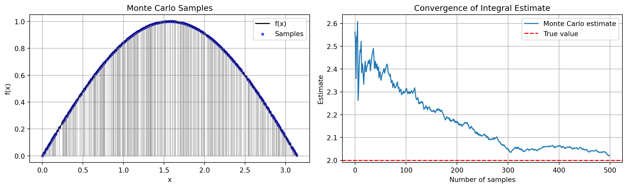
import randomimport mathimport numpy as npimport matplotlib.pyplot as pltdef monte_carlo_integrate_visual_with_sticks(f, a, b, n_samples, seed=None):""" Monte Carlo integration visualization. Shows the function curve, sampled points, and vertical lines ("sticks"). Also plots convergence of the Monte Carlo estimate. """if seed isnotNone: np.random.seed(seed) xs = np.random.uniform(a, b, size=n_samples) ys = f(xs) cumulative_avg = np.cumsum(ys) / np.arange(1, n_samples +1) estimates = (b - a) * cumulative_avg fig, ax = plt.subplots(1, 2, figsize=(13, 4))# ----- Left panel: samples + vertical lines ----- X = np.linspace(a, b, 400) ax[0].plot(X, f(X), color="black", label="f(x)")# Vertical linesfor x_i, y_i inzip(xs, ys): ax[0].plot([x_i, x_i], [0, y_i], color="gray", alpha=0.3, linewidth=1)# Sampled points ax[0].scatter(xs, ys, s=12, color="blue", alpha=0.6, label="Samples") ax[0].set_title("Monte Carlo Samples") ax[0].set_xlabel("x") ax[0].set_ylabel("f(x)") ax[0].grid(True) ax[0].legend()# ----- Right panel: convergence ----- true_value =2.0# ∫₀^π sin(x) dx ax[1].plot(estimates, label="Monte Carlo estimate") ax[1].axhline(true_value, linestyle="--", color="red", label="True value") ax[1].set_title("Convergence of Integral Estimate") ax[1].set_xlabel("Number of samples") ax[1].set_ylabel("Estimate") ax[1].grid(True) ax[1].legend() plt.tight_layout() plt.show()return estimates[-1]def main(): f = np.sin a, b =0.0, math.pi n_samples =500 estimate = monte_carlo_integrate_visual_with_sticks(f, a, b, n_samples, seed=123)print(f"Final estimate ≈ {estimate:.6f} (true = 2.0)")main()
Final estimate ≈ 2.022106 (true = 2.0)
Numerical Integration
Code
def monte_carlo_integrate(f, a, b, n_samples, seed=None):""" Estimate ∫_a^b f(x) dx using simple Monte Carlo integration. Parameters ---------- f : callable Function to integrate. a, b : float Integration bounds (a < b). n_samples : int Number of random samples to draw. seed : int or None Optional seed for reproducibility. Returns ------- estimate : float Monte Carlo estimate of the integral. """if seed isnotNone: random.seed(seed) total =0.0for _ inrange(n_samples): x = random.uniform(a, b) total += f(x)return (b - a) * total / n_samplesdef main():# Example: integrate f(x) = sin(x) on [0, π] f = math.sin a, b =0.0, math.pifor n in [100, 1_000, 10_000, 100_000]: estimate = monte_carlo_integrate(f, a, b, n, seed=0)print(f"n = {n:6d} → estimate ≈ {estimate:.6f} (delta = {abs(2.0- estimate):.6f})")main()
n =    100 → estimate ≈ 2.080957 (delta = 0.080957)
n =   1000 → estimate ≈ 1.992136 (delta = 0.007864)
n =  10000 → estimate ≈ 2.007041 (delta = 0.007041)
n = 100000 → estimate ≈ 1.996149 (delta = 0.003851)