Compromis biais-variance

CSI 4506 - Automne 2025

Marcel Turcotte

Version: sept. 28, 2025 16h07

Préambule

Résumé

Dans cette présentation, nous explorons comment la complexité du modèle influence le biais, la variance, et la généralisation en examinant le sous-ajustement et le sur-ajustement à travers les courbes d’apprentissage pour divers modèles, y compris les modèles linéaires, polynomiaux, basés sur des arbres, KNN et les réseaux profonds.

Résultats d’apprentissage

• Comprendre comment la complexité du modèle affecte le biais, la variance et la généralisation.
• Analyser les courbes d’apprentissage pour diagnostiquer le sous-ajustement et le sur-ajustement.

Complexité du modèle

Justification

L’optimisation de la performance du modèle dépend de manière cruciale de la sélection et du réglage minutieux des hyperparamètres.

Ces hyperparamètres jouent un rôle central dans la régulation de la complexité des modèles d’apprentissage machine.

Définition

La complexité du modèle se réfère à la capacité d’un modèle à capturer des motifs complexes dans les données.

Elle est déterminée par le nombre de paramètres ou la structure du modèle.

Exploration

import numpy as np

np.random.seed(42)

X = 6 * np.random.rand(100, 1) - 3
y = 0.5 * X ** 2 - X + 2 + np.random.randn(100, 1)

import matplotlib as mpl
import matplotlib.pyplot as plt

plt.figure(figsize=(6,4))

plt.plot(X, y, "b.")
plt.xlabel("$x$", fontsize=18)
plt.ylabel("$y$", rotation=0, fontsize=18)
plt.axis([-3, 3, 0, 10])
plt.grid(True)
plt.show()

Dans les expériences d’apprentissage automatique, spécifier le germe du générateur de nombres aléatoires est crucial pour garantir la reproductibilité. En fixant un germe, les programmeurs peuvent garantir que la même séquence de nombres aléatoires sera générée à chaque exécution de l’expérience. Cette cohérence est vitale pour plusieurs raisons :

1. Reproductibilité : Elle permet à d’autres programmeurs de reproduire l’expérience dans les mêmes conditions exactes, facilitant la vérification et la validation des résultats.
2. Analyse comparative : Elle permet une comparaison cohérente entre différents modèles ou algorithmes dans les mêmes conditions initiales, garantissant que les différences observées sont dues aux modèles eux-mêmes plutôt qu’à des variations dans l’initialisation aléatoire.
3. Débogage : Elle aide au débogage en fournissant un environnement stable où les problèmes peuvent être reproduits et étudiés de manière cohérente.

Attribution : Géron (2022), Chapitre 4

Régression linéaire

from sklearn.linear_model import LinearRegression

lin_reg = LinearRegression()
lin_reg.fit(X, y)

X_new = np.array([[-3], [3]])
y_pred = lin_reg.predict(X_new)

plt.figure(figsize=(6,4))

plt.plot(X, y, "b.")
plt.plot(X_new, y_pred, "r-")
plt.xlabel("$x$", fontsize=18)
plt.ylabel("$y$", rotation=0, fontsize=18)
plt.axis([-3, 3, 0, 10])
plt.show()

Un modèle linéaire représente mal cet ensemble de données.

Ajuster la pente conduit invariablement à un scénario où les résidus (erreurs) sont minimisés pour certains points de données tout en restant significatifs pour d’autres.

Définition

L’ingénierie des attributs est le processus de création, transformation et sélection de variables (attributs) à partir de données brutes pour améliorer la performance des modèles d’apprentissage automatique.

Ici, notre objectif est de créer de nouveaux attributs à partir de données brutes.

Ingénierie de l’apprentissage automatique

• Machine Learning Engineering par Andriy Burkov (A. Burkov 2020).
• Couvre la collecte de données, le stockage, le prétraitement, l’ingénierie des attributs, le test et le débogage des modèles, le déploiement, la retraite et la maintenance.
• De l’auteur de Hundred Page Machine Learning Book (Andriy Burkov 2019).
• Disponible sous un modèle “lire d’abord, acheter plus tard”.

PolynomialFeatures

from sklearn.preprocessing import PolynomialFeatures

poly_features = PolynomialFeatures(degree=2, include_bias=False)
X_poly = poly_features.fit_transform(X)

X[0]

array([-0.75275929])

X_poly[0]

array([-0.75275929,  0.56664654])

sklearn.preprocessing.PolynomialFeatures

Générez une nouvelle matrice d’attributs constituée de toutes les combinaisons polynomiales des attributs avec un degré inférieur ou égal au degré spécifié. Par exemple, si un échantillon d’entrée est bidimensionnel et de la forme \([a, b]\), les attributs polynomials de degré 2 sont \([1, a, b, a^2, ab, b^2]\).

PolynomialFeatures

Étant donné deux attributs \(a\) et \(b\), PolynomialFeatures avec degree=3 ajouterait \(a^2\), \(a^3\), \(b^2\), \(b^3\), ainsi que \(ab\), \(a^2b\), \(ab^2\) !

Avertissement

PolynomialFeatures(degree=d) ajoute \(\frac{(D+d)!}{d!D!}\) attributs, où \(D\) est le nombre initial d’attributs.

De plus, vous avez la possibilité de créer vos propres nouveaux attributs.

Régression polynomiale

lin_reg = LinearRegression()
lin_reg = lin_reg.fit(X_poly, y)

X_new = np.linspace(-3, 3, 100).reshape(100, 1)
X_new_poly = poly_features.transform(X_new)
y_new = lin_reg.predict(X_new_poly)

plt.figure(figsize=(5, 3))
plt.plot(X, y, "b.")
plt.plot(X_new, y_new, "r-", linewidth=2, label="Prédictions")
plt.xlabel("$x_1$")
plt.ylabel("$y$", rotation=0)
plt.legend(loc="upper left")
plt.axis([-3, 3, 0, 10])
plt.grid()
plt.show()

LinearRegression sur PolynomialFeatures

lin_reg = LinearRegression()
lin_reg.fit(X_poly, y)

Régression polynomiale

Les données ont été générées selon l’équation suivante, avec l’inclusion de bruit gaussien.

\[ y = 0.5 x^2 - 1.0 x + 2.0 \]

Présenté ci-dessous est le modèle appris.

\[ \hat{y} = 0.56 x^2 + (-1.06) x + 1.78 \]

lin_reg.coef_, lin_reg.intercept_

(array([[-1.06633107,  0.56456263]]), array([1.78134581]))

1. La linéarité concerne les coefficients, pas les entrées brutes

• La régression logistique est linéaire dans ses paramètres (poids).
• La frontière de décision provient de :

\[ \hat{y_i} = \sigma(\theta_0 + \theta_1 z_i^{(1)} + \theta_2 z_i^{(2)} + \dots + \theta_{D'} z_i^{(D')}) \]

où chaque \(z_i^{(j)}\) est un attribut.

• Si vous définissez \(z_i^{(j)}\) comme une fonction polynomiale des variables originales (par exemple \(z_i^{(3)} = (x_i^{(1)})^2\)), le modèle reste linéaire dans les \(z_i^{(j)}\).

2. PolynomialFeatures ne fait que changer l’espace des attributs

• PolynomialFeatures transforme l’entrée \((x_i^{(1)}, x_i^{(2)})\) en un nouveau vecteur : \((x_i^{(1)}, x_i^{(2)}, (x_i^{(1)})^2, x_i^{(1)}x_i^{(2)}, (x_i^{(2)})^2, \ldots)\).
• La régression logistique trouve alors une frontière de décision linéaire dans cet espace d’attributs étendu.
• Lorsque vous le mappez de nouveau à l’espace original \((x_i^{(1)}, x_i^{(2)})\), cette surface de décision “linéaire” peut apparaître courbée ou sinueuse, mais mathématiquement c’est toujours un hyperplan dans l’espace transformé.

Message clé :

“La régression logistique trouve toujours une frontière linéaire dans les attributs que vous lui fournissez. Si vous lui fournissez des polynômes, la frontière linéaire dans cet espace semble non linéaire dans l’espace original.”

Complexité du modèle

from sklearn.preprocessing import StandardScaler
from sklearn.pipeline import make_pipeline

plt.figure(figsize=(5, 3))

for style, width, degree in (("r-+", 2, 1), ("b--", 2, 2), ("g-", 1, 300)):
    polybig_features = PolynomialFeatures(degree=degree, include_bias=False)
    std_scaler = StandardScaler()
    lin_reg = LinearRegression()
    polynomial_regression = make_pipeline(polybig_features, std_scaler, lin_reg)
    polynomial_regression.fit(X, y)
    y_newbig = polynomial_regression.predict(X_new)
    label = f"{degree} degré{'s' if degree > 1 else ''}"
    plt.plot(X_new, y_newbig, style, label=label, linewidth=width)

plt.plot(X, y, "b.", linewidth=3)
plt.legend(loc="upper left")
plt.xlabel("$x_1$")
plt.ylabel("$y$", rotation=0)
plt.axis([-3, 3, 0, 10])
plt.grid()
plt.show()

Une faible valeur de perte sur l’ensemble d’entraînement n’indique pas nécessairement un modèle “meilleur”.

Dans cet exemple, le modèle de régression linéaire présente une erreur quadratique moyenne élevée (perte) sur l’ensemble d’entraînement (ligne rouge). Cela suggère que le modèle commet de nombreuses erreurs même sur les données d’entraînement.

Inversement, le modèle polynomial avec degré=300 montre une erreur quadratique moyenne faible (perte) sur l’ensemble d’entraînement (ligne verte), ce qui implique qu’il commet peu d’erreurs sur les données d’entraînement.

Cependant, le modèle polynomial de degré=300 est susceptible de mal performer sur de futures prédictions. La courbe verte dépasse les limites de l’image sur l’axe des y. Par exemple, pour des valeurs d’entrée dans la plage de 2 à 3, le modèle prédit des valeurs dépassant 10 (ainsi que des valeurs négatives), alors que les valeurs attendues devraient se situer dans la plage de 2 à 4.

Cet exemple illustratif peut sembler simpliste puisque les données sont générées à partir d’une équation quadratique et ne comportent qu’un seul attribut, ce qui rend la visualisation simple. Cependant, il met en évidence un point clé pertinent pour des modèles plus complexes, tels que les réseaux neuronaux profonds. À mesure que le nombre de paramètres augmente, la capacité du modèle à s’adapter aux données d’entraînement augmente également, ce qui peut conduire à un surapprentissage si cela n’est pas correctement géré.

Attribution: 04_training_linear_models.ipynb

Sous- et sur- ajustement

• Sous-ajustement (underfitting):
  • Votre modèle est trop simple (ici, linéaire).
  • Attributs non informatifs.
  • Mauvaise performance sur les données d’entraînement et de test.
• Sur-ajustement (overfitting):
  • Votre modèle est trop complexe (arbre de décision haut, réseaux neuronaux profonds et larges, etc.).
  • Trop d’attributs étant donné le nombre d’exemples disponibles.
  • Excellente performance sur l’ensemble d’entraînement, mais mauvaise performance sur l’ensemble de test.

Un modèle est dit en sous-ajustement lorsqu’il échoue à capturer la structure sous-jacente des données, il performe mal tant sur l’ensemble d’entraînement que sur les données de test non vues. Voici les principales façons dont cela peut se produire :

Capacité du modèle trop faible

• Classe d’hypothèse trop simple : par ex., ajuster une ligne droite (régression linéaire) à des données avec un motif quadratique.
• Architecture peu profonde : utiliser un perceptron monocouche pour une tâche de classification fortement non linéaire.
• Trop peu d’attributs : ne pas fournir suffisamment de variables descriptives au modèle pour capturer le signal.

Trop de régularisation

• Pénalité L2 (ridge) ou L1 (lasso) excessive réduit presque à zéro les coefficients.
• Taux de dropout trop élevé dans les réseaux neuronaux.
• Arrêt prématuré avant que le modèle n’apprenne les motifs.

Problèmes d’optimisation

• Taux d’apprentissage trop petit : le modèle apprend à peine, bloqué avec une perte élevée.
• Taux d’apprentissage trop grand : l’optimiseur oscille, ne converge jamais correctement.
• Trop peu d’époques/itérations d’entraînement : le modèle ne reçoit pas suffisamment de mises à jour pour s’adapter aux données.
• Mauvaise initialisation (surtout dans les problèmes non convexes comme les réseaux profonds) peut entraver la convergence.

Causes liées aux données

• Le bruit des étiquettes domine le signal : si l’ensemble de données est très bruyant, même un bon modèle semble sous-ajuster.
• Volume de données insuffisant : le modèle ne peut pas bien généraliser car l’ensemble d’entraînement ne capture pas la véritable structure.
• Problèmes de mise à l’échelle des attributs : par ex., régression logistique ou réseaux neuronaux entraînés sur des attributs brutes, non mises à l’échelle, mauvaise convergence et ajustement.
• Mauvaise ingénierie des attributs : termes d’interaction manquants, termes polynomiaux, embeddings, etc.

Incompatibilités algorithmiques

• Mauvaise fonction de perte : par ex., utiliser MSE pour une classification fortement déséquilibrée au lieu de la perte logarithmique.
• Choix de modèle incompatible : par ex., k-NN avec k trop grand, prédit presque toujours la classe majoritaire.
• Hypothèse de biais trop forte : par ex., Naive Bayes supposant l’indépendance des attributs alors qu’elle est fortement violée.

Résumé :

Le sous-ajustement se produit lorsque le modèle est trop contraint (faible capacité, trop de régularisation, trop peu d’entraînement) ou lorsque le processus d’entraînement échoue (problèmes d’optimisation/données). On le remarque généralement lorsque la perte d’entraînement reste élevée même après un long entraînement.

Un modèle sur-ajuste lorsqu’il apprend non seulement la structure sous-jacente des données d’entraînement mais aussi le bruit et les idiosyncrasies, ce qui conduit à une mauvaise généralisation sur les données non vues. Voici les principales façons dont cela peut se produire :

Capacité du modèle trop élevée

• Modèle trop flexible (par ex., réseau neuronal très profond sur un petit ensemble de données).
• Trop d’attributs par rapport au nombre d’échantillons → haute variance.
• Ajouter des attributs polynomiaux de haut degré sans suffisamment de données.

Trop peu de régularisation

• Pénalité L1/L2 faible ou inexistante permet aux poids de devenir très grands.
• Taux de dropout trop faible ou désactivé.

Entraînement trop long

• Le modèle continue de minimiser la perte d’entraînement bien au-delà du point où la perte de validation atteint son minimum.
• Pas d’arrêt précoce → mémorisation du bruit/des valeurs aberrantes.

Problèmes de données

• L’ensemble d’entraînement est trop petit, le modèle mémorise au lieu de généraliser.
• Bruit d’étiquettes élevé, le modèle s’ajuste aux erreurs.
• Fuite d’informations de test dans l’entraînement (par ex., prétraitement, mise à l’échelle ou construction d’attributs inadéquats).

Incompatibilité d’évaluation

• Hyperparamètres ajustés directement sur l’ensemble de test, le modèle s’adapte à cet ensemble de test plutôt qu’à la distribution sous-jacente.
• Les plis de validation croisée ne sont pas stratifiés, signaux de généralisation trompeurs.

Choix algorithmiques

• k-NN avec k=1 (mémorise les points d’entraînement).
• Arbre de décision sans profondeur maximale ni élagage.
• Réseau neuronal avec trop de paramètres par rapport à la taille du jeu de données.

Résumé :

Le sur-ajustement se produit lorsque le modèle a trop de liberté, trop peu de contraintes, ou s’entraîne trop longtemps sur un ensemble de données limité/bruyant. On le reconnaît lorsque la perte d’entraînement est très basse mais la perte de validation/test est beaucoup plus élevée.

Courbes d’apprentissage

• Une façon d’évaluer nos modèles est de visualiser les courbes d’apprentissage :
  • Une courbe d’apprentissage montre la performance de notre modèle, ici en utilisant la RMSE, à la fois sur le jeu d’entraînement et le jeu de test.
  • Plusieurs mesures sont obtenues en entraînant le modèle de manière répétée sur des sous-ensembles de données de plus en plus grands.

Voir : sklearn.model_selection.learning_curve.

Courbe d’apprentissage – Sous-ajustement

from sklearn.model_selection import learning_curve

train_sizes, train_scores, valid_scores = learning_curve(
    LinearRegression(), X, y, train_sizes=np.linspace(0.01, 1.0, 40), cv=5,
    scoring="neg_root_mean_squared_error")

train_errors = -train_scores.mean(axis=1)
valid_errors = -valid_scores.mean(axis=1)

plt.figure(figsize=(6, 4))  # code supplémentaire – non nécessaire, juste pour le formatage
plt.plot(train_sizes, train_errors, "r-+", linewidth=2, label="train")
plt.plot(train_sizes, valid_errors, "b-", linewidth=3, label="test")

# code supplémentaire – embellit
plt.xlabel("Taille du jeu d'entraînement")
plt.ylabel("RMSE")
plt.grid()
plt.legend(loc="upper right")
plt.axis([0, 80, 0, 2.5])
plt.show()

• Polynôme avec degré=1.

• Performance médiocre sur les données de formation et de test.

Ce graphique illustre la courbe d’apprentissage pour un modèle de régression linéaire appliqué à des données générées à partir d’une équation quadratique, qui sert d’exemple continu.

L’axe horizontal représente la taille du jeu d’entraînement. Initialement, le modèle de régression linéaire est entraîné sur un très petit jeu de données, composé d’un ou de quelques exemples, et l’erreur quadratique moyenne (RMSE) est tracée pour les ensembles de formation et de test. La taille du jeu d’entraînement est ensuite augmentée progressivement, un nouveau modèle est entraîné, et la performance est enregistrée. Cette procédure continue jusqu’à ce que l’ensemble du jeu de données soit utilisé.

Les observations clés du graphique incluent :

• Avec un ou deux exemples seulement, le modèle s’ajuste parfaitement au jeu d’entraînement, résultant en un faible RMSE pour les données d’entraînement.

• À mesure que la taille du jeu d’entraînement augmente, le modèle a du mal à s’ajuster aux données d’entraînement en raison de la nature quadratique du processus de génération de données. Par conséquent, le RMSE pour le jeu d’entraînement augmente et se stabilise à un niveau plus élevé.

• Pour les petits jeux d’entraînement, le modèle fonctionne mal sur le jeu de test en raison d’une généralisation inadéquate, ce qui entraîne un RMSE élevé.

• À mesure que la taille du jeu d’entraînement augmente, la performance sur le jeu de test s’améliore, indiquée par une diminution du RMSE, jusqu’à atteindre un point où de nouvelles augmentations de la taille du jeu d’entraînement n’apportent pas d’améliorations significatives.

Ces courbes d’apprentissage sont indicatives d’un modèle qui sous-ajuste. Les courbes de RMSE pour les ensembles de formation et de test se stabilisent à des valeurs relativement élevées et restent proches l’une de l’autre, comme le note Géron (2022).

Code source: 04_training_linear_models.ipynb.

Courbe d’apprentissage – Surapprentissage

from sklearn.pipeline import make_pipeline

polynomial_regression = make_pipeline(
    PolynomialFeatures(degree=14, include_bias=False),
    LinearRegression())

train_sizes, train_scores, valid_scores = learning_curve(
    polynomial_regression, X, y, train_sizes=np.linspace(0.01, 1.0, 40), cv=5,
    scoring="neg_root_mean_squared_error")
# code supplémentaire – génère et enregistre la Figure 4–16

train_errors = -train_scores.mean(axis=1)
valid_errors = -valid_scores.mean(axis=1)

plt.figure(figsize=(6, 4))
plt.plot(train_sizes, train_errors, "r-+", linewidth=2, label="train")
plt.plot(train_sizes, valid_errors, "b-", linewidth=3, label="test")
plt.legend(loc="upper right")
plt.xlabel("Taille de l'ensemble d'entraînement")
plt.ylabel("RMSE")
plt.grid()
plt.axis([0, 80, 0, 2.5])
plt.show()

• Polynôme avec degré=14.

• Performance excellente sur l’ensemble d’entraînement, mais performance médiocre sur l’ensemble de test.

• Pour un ensemble d’entraînement allant jusqu’à 14 points de données, le polynôme s’ajuste parfaitement aux données d’entraînement, entraînant un RMSE de zéro.

• L’erreur sur les données d’entraînement dans ce cas est significativement plus basse.

• Un écart notable entre les deux courbes indique que le modèle fonctionne nettement mieux sur les données d’entraînement par rapport aux données de test.

Surapprentissage - Réseaux profonds

Les réseaux de neurones seront abordés en détail plus tard dans notre cours. Le graphique présenté ici illustre la variation de la fonction de perte au fur et à mesure qu’un modèle d’apprentissage profond s’entraîne.

Cet exemple utilise le jeu de données de classification de sentiments des critiques de films IMDB disponible dans Keras. Le jeu de données comprend 25 000 critiques de films provenant d’IMDB, chacune étant étiquetée avec un sentiment (positif ou négatif).

Le modèle se compose de trois couches denses de tailles 16, 16 et 1, respectivement. Il inclut un total de 160 305 paramètres entraînables.

Le réseau est entraîné en utilisant la descente de gradient stochastique par mini-lots avec une taille de lot de 512. L’axe horizontal représente le nombre d’époques, où chaque époque indique que le modèle a vu l’ensemble d’entraînement une fois. Au cours de chaque époque, l’algorithme de descente de gradient stochastique met à jour les paramètres du modèle de manière itérative en utilisant des mini-lots de 512 exemples.

J’ai choisi cet exemple pour illustrer qu’un réseau de neurones avec une capacité suffisante (nombre de paramètres) peut minimiser les erreurs d’entraînement presque à zéro, car réduire l’erreur d’entraînement est l’objectif principal de l’optimisation. Cependant, le graphique démontre clairement qu’au-delà d’un certain point, les motifs appris deviennent spécifiques au jeu d’entraînement plutôt que des principes généraux. La généralisation, plutôt que la simple mémorisation, est l’objectif ultime de l’apprentissage automatique.

Le surapprentissage se produit lorsqu’un modèle apprend les détails et le bruit dans les données d’entraînement à un point tel que cela impacte négativement la performance du modèle sur de nouvelles données. Cela peut entraîner une frontière de décision qui s’adapte trop étroitement aux données d’entraînement, capturant du bruit et des détails non pertinents plutôt que des motifs généraux.

Exemple tiré de Chollet (2017) Chapitre 3 (chapter04_getting-started-with-neural-networks.ipynb, ipynb de l’édition 2021).

Surapprentissage - Réseau profond

Ce graphique illustre de manière similaire la variation de l’exactitude pour les ensembles d’entraînement et de test au fur et à mesure que le modèle subit l’entraînement.

Compromis biais-variance

Biais

• Biais fait référence à l’erreur introduite en approximant un problème du monde réel, qui peut être complexe, en utilisant un modèle simplifié.

• Il représente la différence entre la prédiction moyenne du modèle et le résultat vrai.

• Un biais élevé peut amener un algorithme à manquer des motifs importants, conduisant à un sous-ajustement.

Biais

\[ \text{Biais}(\hat{f}) = \mathbb{E}[\hat{f}(x)] - f(x) \] où :

• \(\hat{f}(x)\) est la prédiction faite par le modèle,
• \(f(x)\) est la fonction vraie,
• \(\mathbb{E}[\hat{f}(x)]\) est la prédiction attendue sur différents ensembles de données.

Variance

• Variance mesure la sensibilité du modèle aux fluctuations dans les données d’entraînement.

• Une variance élevée indique que le modèle capture le bruit comme s’il s’agissait d’un vrai motif, conduisant à un surdéajustement.

• Elle reflète combien les prédictions du modèle varieraient si différentes données d’entraînement étaient utilisées.

Variance

\[ \text{Variance}(\hat{f}) = \mathbb{E}[(\hat{f}(x) - \mathbb{E}[\hat{f}(x)])^2] \]

où :

• \(\hat{f}(x)\) est la prédiction faite par le modèle,
• \(\mathbb{E}[\hat{f}(x)]\) est la prédiction attendue sur différents ensembles de données.

Remarques

• L’apprentissage statistique fait des hypothèses sur le modèle, la distribution des données et le bruit pour dériver analytiquement les valeurs attendues.

• Dans les applications pratiques, des techniques empiriques comme la validation croisée et le bootstrapping sont utilisées pour estimer le biais et la variance.

Compromis biais-variance

\[ \text{Erreur} = \text{Biais}^2 + \text{Variance} + \text{Erreur Irréductible} \]

• La sélection de modèle vise à minimiser le biais, qui provient de modèles trop simplistes, et la variance, qui résulte de modèles trop complexes sujets au surapprentissage.

• Idéalement, avec des données infinies, à la fois le biais et la variance pourraient être réduits à zéro.

• Cependant, en pratique, les données sont généralement bruitées, et une certaine erreur irréductible persiste en raison de facteurs non pris en compte au-delà de la portée du modèle.

Visez une complexité de modèle qui capture les motifs essentiels sans tomber dans le surapprentissage.

Compromis biais-variance

Attribution : Bigbossfarin, CC0, via Wikimedia Commons

Compromis biais-variance

Attribution : Understanding the Bias-Variance Tradeoff par Scott Fortmann-Roe, juin 2012.

Biais élevé, faible variance

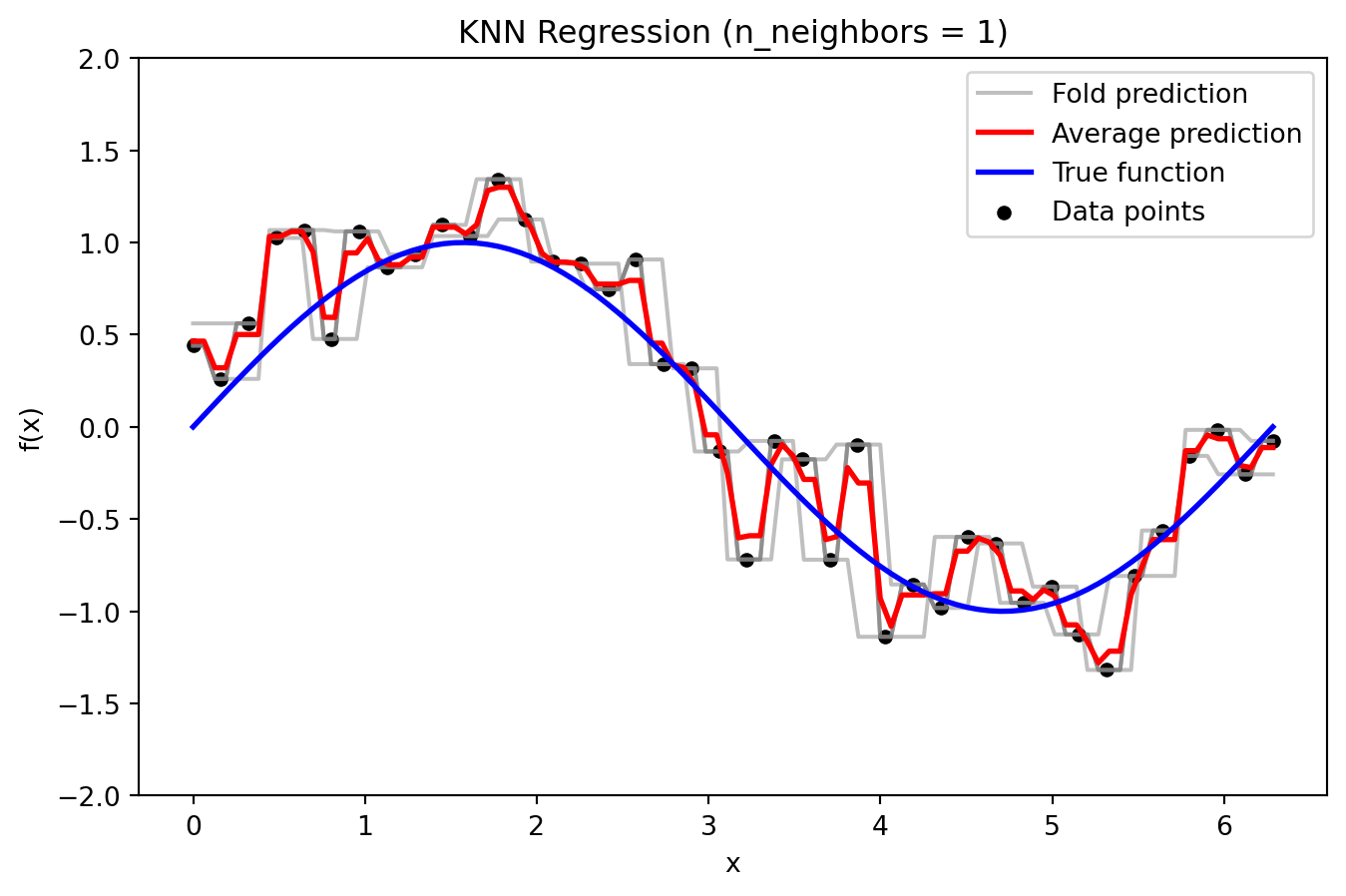
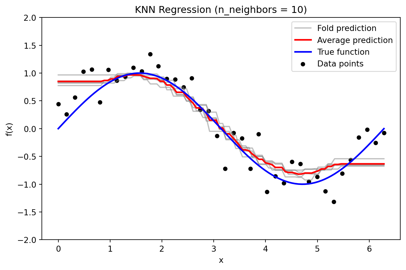
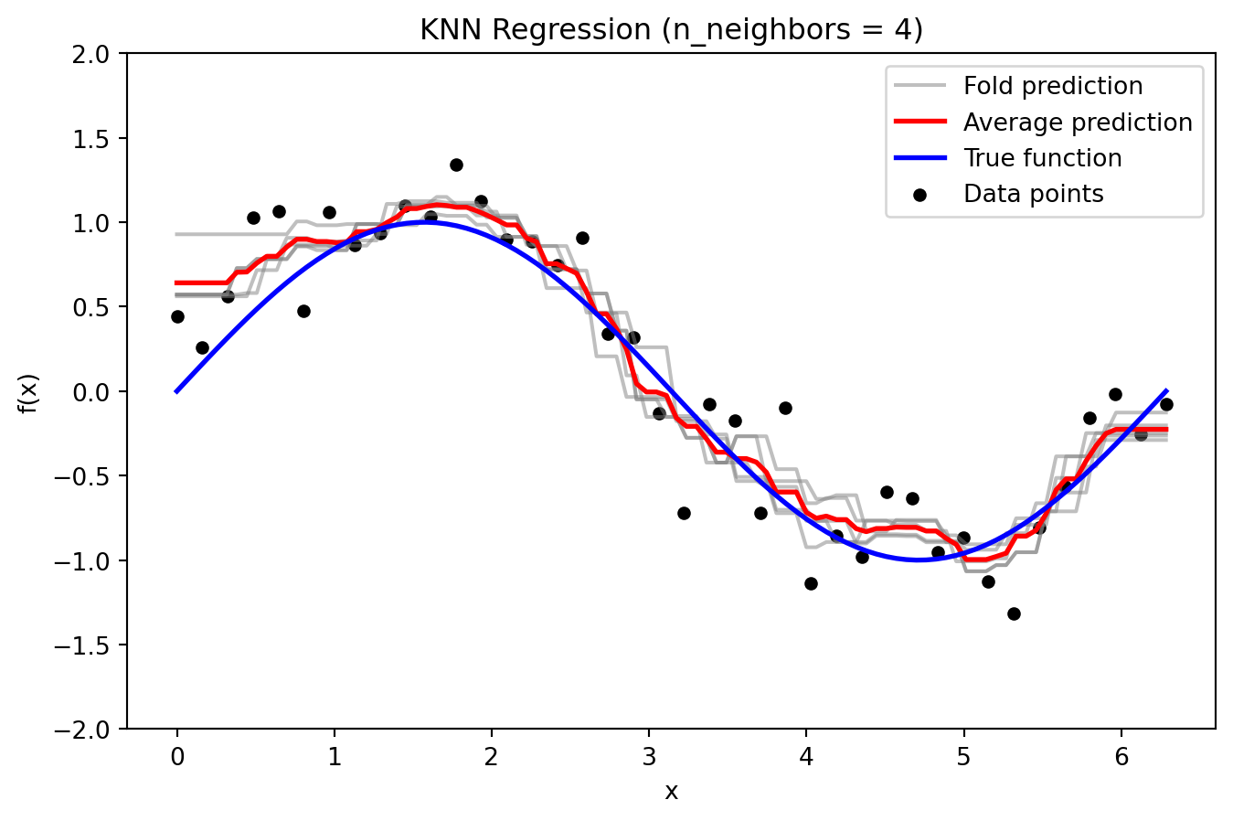
from sklearn.model_selection import KFold
from sklearn.metrics import mean_squared_error

def true_function(x):
    return np.sin(x)

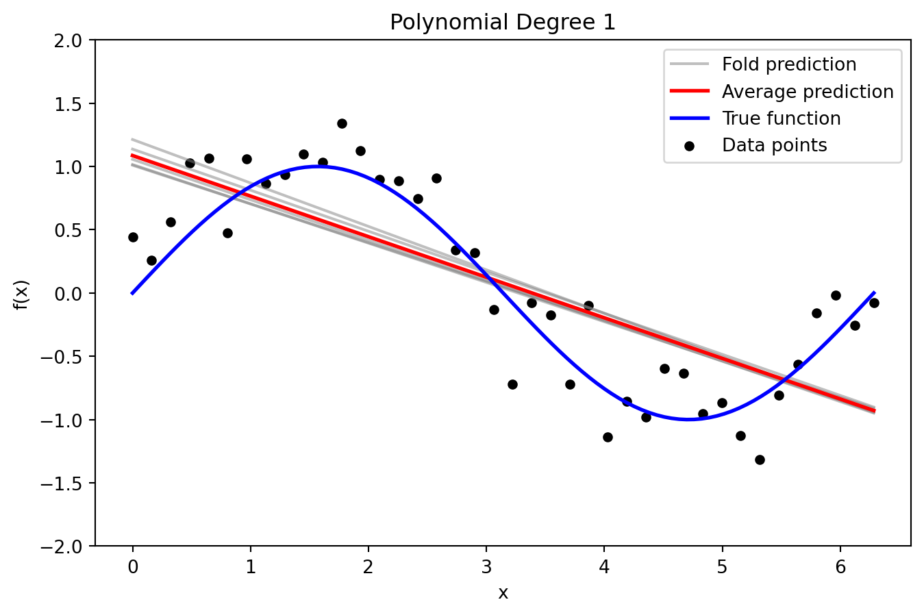
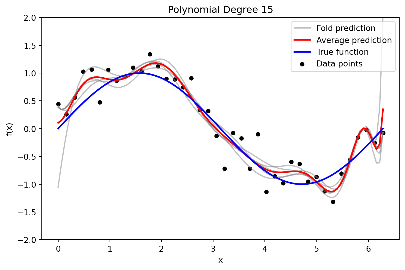
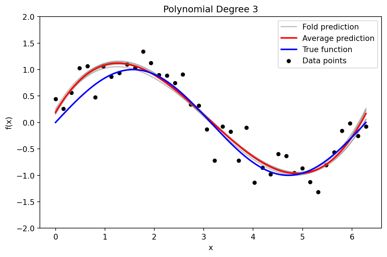
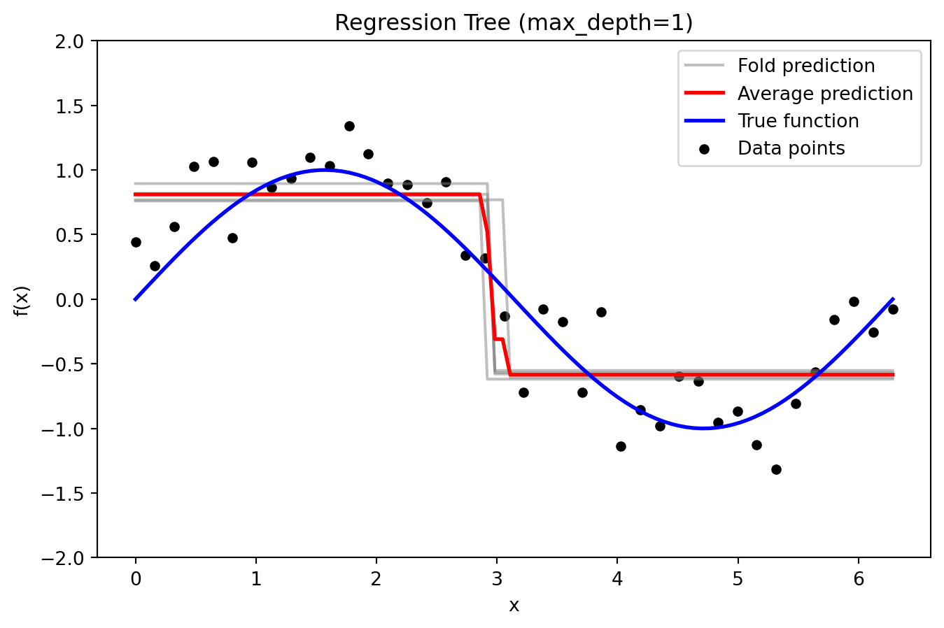
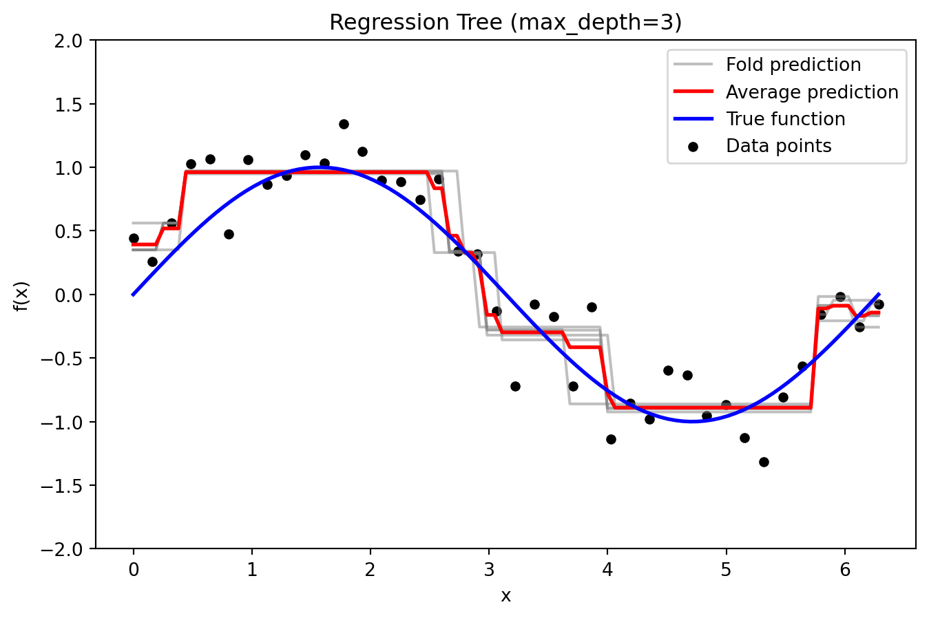
def plot_fold_predictions(degree, X, y, X_grid, y_true_grid, n_splits=5, random_state=42):
    """
    For a given polynomial degree, perform KFold cross-validation,
    plot the individual fold predictions along with the average prediction 
    and the true function (with y-axis limited to [-2, 2]),
    and return predictions and errors.
    """
    kf = KFold(n_splits=n_splits, shuffle=True, random_state=random_state)
    fold_predictions = []  # To store predictions on the evaluation grid for each fold
    fold_errors = []       # To store test errors for each fold

    for train_index, test_index in kf.split(X):
        poly = PolynomialFeatures(degree=degree)
        X_train_poly = poly.fit_transform(X[train_index])
        X_test_poly = poly.transform(X[test_index])
        X_grid_poly = poly.transform(X_grid)
        
        model = LinearRegression()
        model.fit(X_train_poly, y[train_index])
        
        # Predictions on the dense grid for bias-variance analysis
        y_pred_grid = model.predict(X_grid_poly)
        fold_predictions.append(y_pred_grid)
        
        # Test error on held-out data
        y_pred_test = model.predict(X_test_poly)
        fold_errors.append(mean_squared_error(y[test_index], y_pred_test))
    
    fold_predictions = np.array(fold_predictions)
    avg_prediction = np.mean(fold_predictions, axis=0)
    
    # Plot individual fold predictions with y-axis limited to [-2, 2]
    plt.figure(figsize=(8, 5))
    for i in range(n_splits):
        plt.plot(X_grid, fold_predictions[i], color='gray', alpha=0.5, 
                 label='Fold prediction' if i == 0 else "")
    plt.plot(X_grid, avg_prediction, color='red', linewidth=2, label='Average prediction')
    plt.plot(X_grid, y_true_grid, color='blue', linewidth=2, label='True function')
    plt.scatter(X, y, color='black', s=20, label='Data points')
    plt.ylim(-2, 2)
    plt.title(f'Polynomial Degree {degree}')
    plt.xlabel('x')
    plt.ylabel('f(x)')
    plt.legend()
    plt.show()
    
    return fold_predictions, avg_prediction, fold_errors

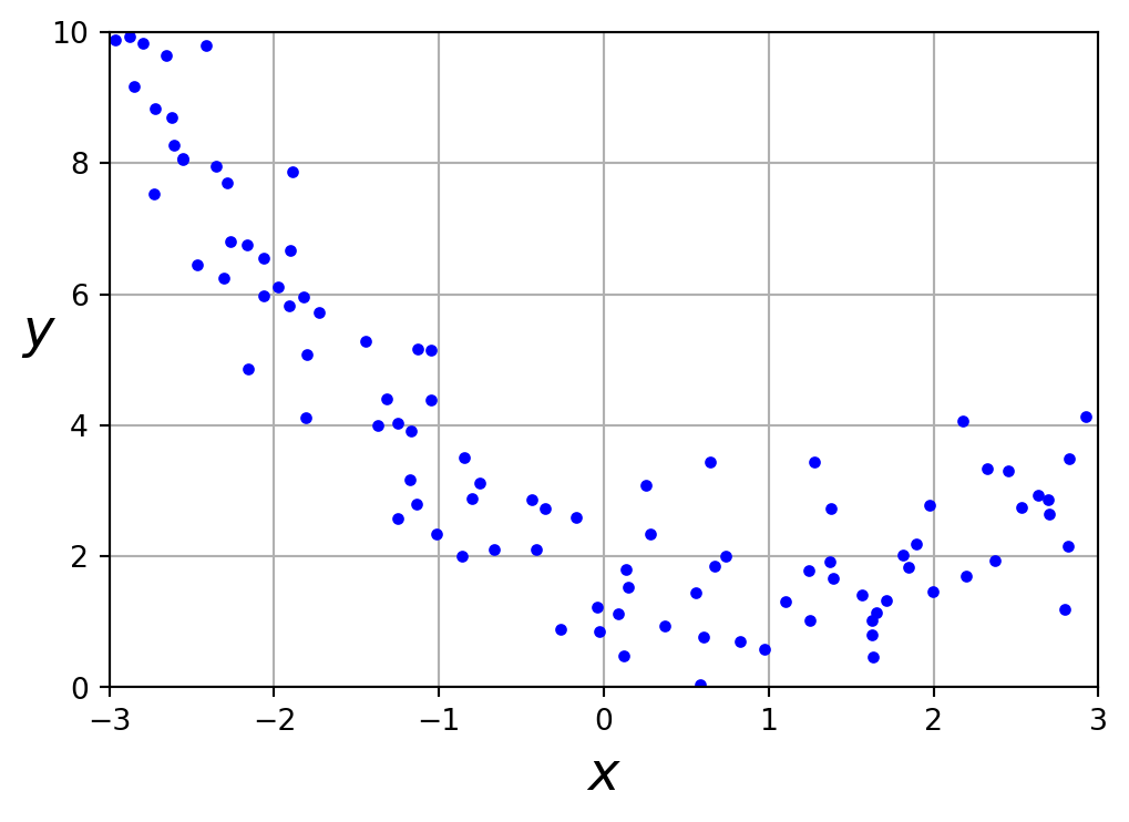
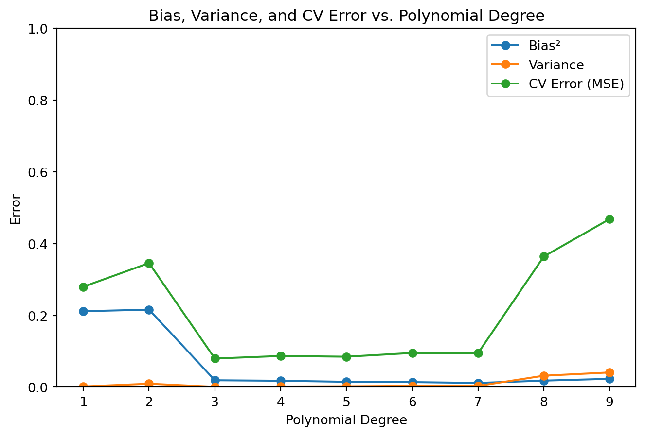
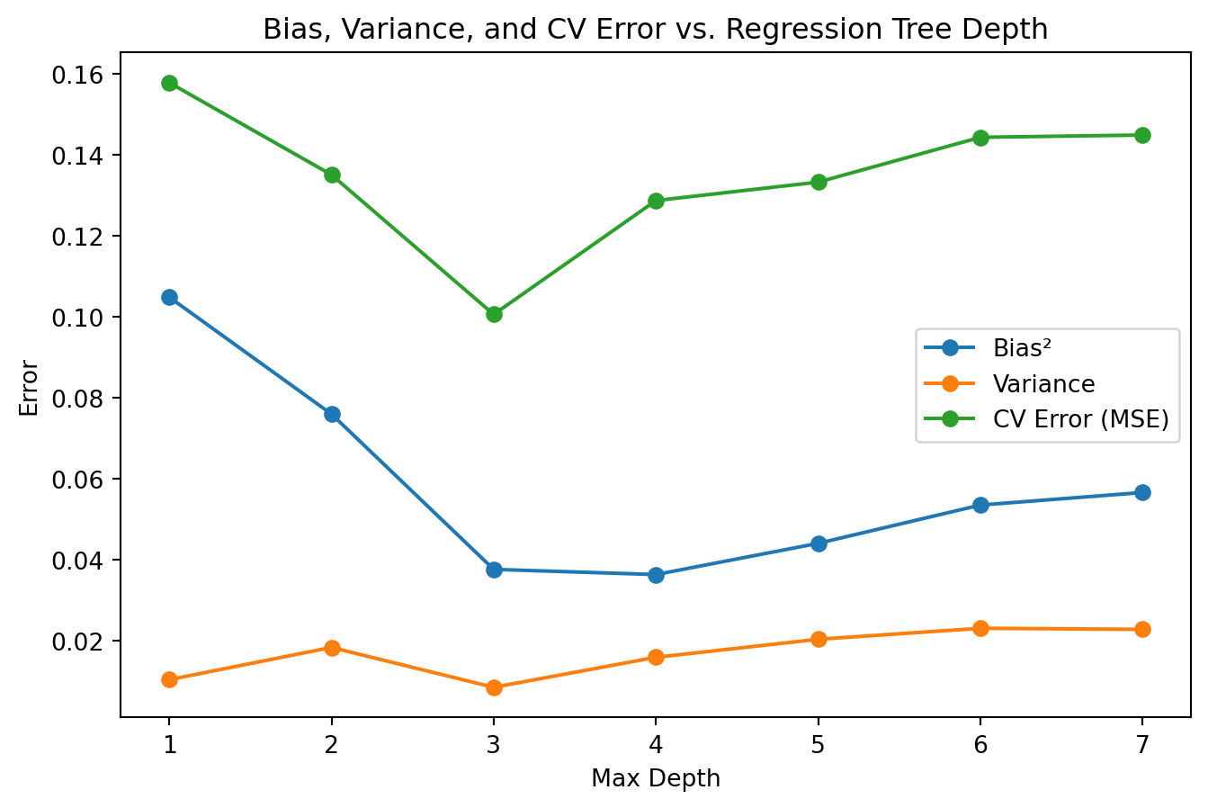
# --- Data Generation with Increased Noise and Reduced Sample Size ---
np.random.seed(0)
n_samples = 40  # Reduced sample size increases model sensitivity to training data
X = np.linspace(0, 2 * np.pi, n_samples).reshape(-1, 1)
noise_std = 0.25  # Increased noise level amplifies prediction variability
y = true_function(X).ravel() + np.random.normal(0, noise_std, size=n_samples)

# Create a dense evaluation grid and compute the true function values
X_grid = np.linspace(0, 2 * np.pi, 100).reshape(-1, 1)
y_true_grid = true_function(X_grid).ravel()

# --- Plot Individual Fold Predictions for Selected Degrees ---
_ = plot_fold_predictions(1, X, y, X_grid, y_true_grid, n_splits=5)

• Biais élevé : Le modèle manque de complexité et, par conséquent, ne parvient pas à capturer les motifs sous-jacents dans les données, ce qui entraîne une erreur moyenne élevée.

• Faible variance : Le modèle montre une insensibilité aux variations dans l’ensemble de données, ce qui se traduit par une faible variance.

Biais faible, variance élevée

_ = plot_fold_predictions(15, X, y, X_grid, y_true_grid, n_splits=5)

Parfait

_ = plot_fold_predictions(3, X, y, X_grid, y_true_grid, n_splits=5)

Biais, variance et erreur de validation

# --- Compute Bias², Variance, and CV Error Across Degrees 1 to 10 ---
degrees = range(1, 10)
bias_list = []
variance_list = []
cv_error_list = []

for degree in degrees:
    kf = KFold(n_splits=5, shuffle=True, random_state=42)
    fold_predictions = []
    fold_errors = []
    
    for train_index, test_index in kf.split(X):
        poly = PolynomialFeatures(degree=degree)
        X_train_poly = poly.fit_transform(X[train_index])
        X_test_poly = poly.transform(X[test_index])
        X_grid_poly = poly.transform(X_grid)
        
        model = LinearRegression()
        model.fit(X_train_poly, y[train_index])
        
        y_pred_grid = model.predict(X_grid_poly)
        fold_predictions.append(y_pred_grid)
        
        y_pred_test = model.predict(X_test_poly)
        fold_errors.append(mean_squared_error(y[test_index], y_pred_test))
    
    fold_predictions = np.array(fold_predictions)
    mean_prediction = np.mean(fold_predictions, axis=0)
    
    # Bias²: Average squared difference between the average prediction and the true function
    bias_sq = np.mean((mean_prediction - y_true_grid)**2)
    # Variance: Average variance of the predictions across the evaluation grid
    variance = np.mean(np.var(fold_predictions, axis=0))
    # CV Error: Mean of the MSE on held-out test sets
    cv_error = np.mean(fold_errors)
    
    bias_list.append(bias_sq)
    variance_list.append(variance)
    cv_error_list.append(cv_error)

# --- Plot Bias², Variance, and CV Error vs. Polynomial Degree ---
plt.figure(figsize=(8, 5))
plt.plot(degrees, bias_list, marker='o', label='Bias²')
plt.plot(degrees, variance_list, marker='o', label='Variance')
plt.plot(degrees, cv_error_list, marker='o', label='CV Error (MSE)')
plt.title('Bias, Variance, and CV Error vs. Polynomial Degree')
plt.xlabel('Polynomial Degree')
plt.ylabel('Error')
plt.ylim(0, 1)
plt.legend()
plt.show()

Abre de décision

from sklearn.tree import DecisionTreeRegressor

def plot_tree_fold_predictions(max_depth, X, y, X_grid, y_true_grid, n_splits=5, random_state=42):
    """
    For a given tree max_depth, perform KFold cross-validation with a DecisionTreeRegressor,
    plot the individual fold predictions along with the average prediction and the true function.
    The y-axis is limited to [-2, 2] for clarity.
    """
    kf = KFold(n_splits=n_splits, shuffle=True, random_state=random_state)
    fold_predictions = []  # Store predictions on the evaluation grid for each fold
    fold_errors = []       # Store test errors for each fold

    for train_index, test_index in kf.split(X):
        X_train = X[train_index]
        X_test = X[test_index]
        
        model = DecisionTreeRegressor(max_depth=max_depth, random_state=random_state)
        model.fit(X_train, y[train_index])
        
        # Prediction on a dense evaluation grid
        y_pred_grid = model.predict(X_grid)
        fold_predictions.append(y_pred_grid)
        
        # Test error on held-out data
        y_pred_test = model.predict(X_test)
        fold_errors.append(mean_squared_error(y[test_index], y_pred_test))
    
    fold_predictions = np.array(fold_predictions)
    avg_prediction = np.mean(fold_predictions, axis=0)
    
    plt.figure(figsize=(8, 5))
    for i in range(n_splits):
        plt.plot(X_grid, fold_predictions[i], color='gray', alpha=0.5,
                 label='Fold prediction' if i == 0 else "")
    plt.plot(X_grid, avg_prediction, color='red', linewidth=2, label='Average prediction')
    plt.plot(X_grid, y_true_grid, color='blue', linewidth=2, label='True function')
    plt.scatter(X, y, color='black', s=20, label='Data points')
    plt.ylim(-2, 2)
    plt.title(f'Regression Tree (max_depth={max_depth})')
    plt.xlabel('x')
    plt.ylabel('f(x)')
    plt.legend()
    plt.show()
    
    return fold_predictions, avg_prediction, fold_errors

# --- Plot Individual Fold Predictions for Selected Tree Depths ---
_ = plot_tree_fold_predictions(1, X, y, X_grid, y_true_grid, n_splits=5)

Arbre de décision

_ = plot_tree_fold_predictions(10, X, y, X_grid, y_true_grid, n_splits=5)

Arbre de décision

_ = plot_tree_fold_predictions(3, X, y, X_grid, y_true_grid, n_splits=5)

Biais, variance et erreur de validation

# --- Compute Bias², Variance, and CV Error vs. Tree Depth ---
max_depths = range(1, 8)
bias_list = []
variance_list = []
cv_error_list = []

for depth in max_depths:
    kf = KFold(n_splits=5, shuffle=True, random_state=42)
    fold_predictions = []
    fold_errors = []
    
    for train_index, test_index in kf.split(X):
        X_train = X[train_index]
        X_test = X[test_index]
        
        model = DecisionTreeRegressor(max_depth=depth, random_state=42)
        model.fit(X_train, y[train_index])
        
        y_pred_grid = model.predict(X_grid)
        fold_predictions.append(y_pred_grid)
        
        y_pred_test = model.predict(X_test)
        fold_errors.append(mean_squared_error(y[test_index], y_pred_test))
    
    fold_predictions = np.array(fold_predictions)
    mean_prediction = np.mean(fold_predictions, axis=0)
    
    # Bias²: Mean squared difference between the average prediction and the true function
    bias_sq = np.mean((mean_prediction - y_true_grid)**2)
    # Variance: Average variance of predictions across the evaluation grid
    variance = np.mean(np.var(fold_predictions, axis=0))
    # CV Error: Average test error over folds
    cv_error = np.mean(fold_errors)
    
    bias_list.append(bias_sq)
    variance_list.append(variance)
    cv_error_list.append(cv_error)

plt.figure(figsize=(8, 5))
plt.plot(max_depths, bias_list, marker='o', label='Bias²')
plt.plot(max_depths, variance_list, marker='o', label='Variance')
plt.plot(max_depths, cv_error_list, marker='o', label='CV Error (MSE)')
plt.title('Bias, Variance, and CV Error vs. Regression Tree Depth')
plt.xlabel('Max Depth')
plt.ylabel('Error')
# plt.ylim(0, 1)
plt.legend()
plt.show()

KNN Regression

from sklearn.neighbors import KNeighborsRegressor

def plot_knn_fold_predictions(n_neighbors, X, y, X_grid, y_true_grid, n_splits=5, random_state=42):
    """
    For a given number of neighbors, perform KFold cross-validation using KNeighborsRegressor,
    plot the predictions from each fold along with the average prediction and the true function.
    The y-axis is limited to [-2, 2] for clarity.
    """
    kf = KFold(n_splits=n_splits, shuffle=True, random_state=random_state)
    fold_predictions = []  # Store predictions on the evaluation grid for each fold
    fold_errors = []       # Store test errors for each fold

    for train_index, test_index in kf.split(X):
        X_train = X[train_index]
        X_test = X[test_index]
        
        model = KNeighborsRegressor(n_neighbors=n_neighbors)
        model.fit(X_train, y[train_index])
        
        # Prediction on a dense evaluation grid for bias-variance analysis
        y_pred_grid = model.predict(X_grid)
        fold_predictions.append(y_pred_grid)
        
        # Test error on held-out data
        y_pred_test = model.predict(X_test)
        fold_errors.append(mean_squared_error(y[test_index], y_pred_test))
    
    fold_predictions = np.array(fold_predictions)
    avg_prediction = np.mean(fold_predictions, axis=0)
    
    # Plot individual fold predictions
    plt.figure(figsize=(8, 5))
    for i in range(n_splits):
        plt.plot(X_grid, fold_predictions[i], color='gray', alpha=0.5,
                 label='Fold prediction' if i == 0 else "")
    plt.plot(X_grid, avg_prediction, color='red', linewidth=2, label='Average prediction')
    plt.plot(X_grid, y_true_grid, color='blue', linewidth=2, label='True function')
    plt.scatter(X, y, color='black', s=20, label='Data points')
    plt.ylim(-2, 2)
    plt.title(f'KNN Regression (n_neighbors = {n_neighbors})')
    plt.xlabel('x')
    plt.ylabel('f(x)')
    plt.legend()
    plt.show()
    
    return fold_predictions, avg_prediction, fold_errors

# --- Plot Individual Fold Predictions for Selected Values of k ---
_ = plot_knn_fold_predictions(1, X, y, X_grid, y_true_grid, n_splits=5)

KNN Regression

_ = plot_knn_fold_predictions(10, X, y, X_grid, y_true_grid, n_splits=5)

KNN Regression

_ = plot_knn_fold_predictions(4, X, y, X_grid, y_true_grid, n_splits=5)

Biais, variance et erreur de validation

# --- Compute Bias², Variance, and CV Error vs. Number of Neighbors ---
neighbors_range = range(1, 21)  # Vary k from 1 to 20
bias_list = []
variance_list = []
cv_error_list = []

for k in neighbors_range:
    kf = KFold(n_splits=5, shuffle=True, random_state=42)
    fold_predictions = []
    fold_errors = []
    
    for train_index, test_index in kf.split(X):
        X_train = X[train_index]
        X_test = X[test_index]
        
        model = KNeighborsRegressor(n_neighbors=k)
        model.fit(X_train, y[train_index])
        
        y_pred_grid = model.predict(X_grid)
        fold_predictions.append(y_pred_grid)
        
        y_pred_test = model.predict(X_test)
        fold_errors.append(mean_squared_error(y[test_index], y_pred_test))
    
    fold_predictions = np.array(fold_predictions)
    mean_prediction = np.mean(fold_predictions, axis=0)
    
    # Bias²: Mean squared difference between the average prediction and the true function
    bias_sq = np.mean((mean_prediction - y_true_grid)**2)
    # Variance: Average variance of predictions across the evaluation grid
    variance = np.mean(np.var(fold_predictions, axis=0))
    # CV Error: Average MSE on the held-out test sets
    cv_error = np.mean(fold_errors)
    
    bias_list.append(bias_sq)
    variance_list.append(variance)
    cv_error_list.append(cv_error)

# --- Plot Bias², Variance, and CV Error vs. Number of Neighbors ---
plt.figure(figsize=(8, 5))
plt.plot(neighbors_range, bias_list, marker='o', label='Bias²')
plt.plot(neighbors_range, variance_list, marker='o', label='Variance')
plt.plot(neighbors_range, cv_error_list, marker='o', label='CV Error (MSE)')
plt.title('Bias, Variance, and CV Error vs. Number of Neighbors (KNN)')
plt.xlabel('Number of Neighbors')
plt.ylabel('Error')
# plt.ylim(0, 1)
plt.legend()
plt.show()

Au début, cela peut sembler contre-intuitif, mais c’est une conséquence directe de la manière dont fonctionne le KNN.

Avec un \(k\) très bas (par exemple, \(k = 1\)), le modèle fait des prédictions basées sur le voisin le plus proche, capturant presque tous les détails des données d’entraînement—cela entraîne un biais faible mais une variance élevée car les prédictions sont très sensibles au bruit.

En revanche, un \(k\) plus élevé force le régresseur à faire la moyenne sur de nombreux voisins, ce qui lisse les prédictions. Cela donne un modèle plus simple, moins flexible, qui pourrait ne pas capturer les nuances locales (biais élevé) mais est moins sensible aux fluctuations dans l’ensemble d’entraînement (variance faible).

Comment expliquez-vous que le biais\(^2\) augmente avec la valeur de \(k\) ?

Prologue

Résumé

• Évaluation de la complexité des modèles et de son impact sur la performance.
• Illustration du sous-ajustement, du sur-ajustement, et du compromis biais-variance.
• Démonstration des courbes d’apprentissage et de la validation croisée à travers divers modèles (linéaire, polynomial, arbre, KNN, réseaux profonds).

Prochain cours

• Ingénierie de l’apprentissage automatique

Références

Burkov, A. 2020. Machine Learning Engineering. True Positive Incorporated. https://books.google.ca/books?id=HeXizQEACAAJ.

Burkov, Andriy. 2019. The Hundred-Page Machine Learning Book. Andriy Burkov.

Chollet, François. 2017. Deep learning with Python. Manning Publications.

Géron, Aurélien. 2022. Hands-on Machine Learning with Scikit-Learn, Keras, and TensorFlow. 3ᵉ éd. O’Reilly Media, Inc.

Russell, Stuart, et Peter Norvig. 2020. Artificial Intelligence: A Modern Approach. 4ᵉ éd. Pearson. http://aima.cs.berkeley.edu/.

Marcel Turcotte

Marcel.Turcotte@uOttawa.ca

École de science informatique et de génie électrique (SIGE)

Université d’Ottawa