Definitions, Paradigms, and Tasks
CSI 5180 - Machine Learning for Bioinformatics
Version: Feb 6, 2025 10:53
Preamble
Quote of the Day
Mark Your Calendar
Distinguished Lecture
Leland McInnes, author of UMAP, on April 7, 2025, at 1:30 p.m.
Summary
In this lecture, we will introduce concepts essential for understanding machine learning, including the paradigms (types) and tasks (problems).
General Objective:
- Describe the fundamental concepts of machine learning
Learning Outcomes
- Identify the key components of a learning problem (data, tasks, and performance measures).
- Differentiate between major machine learning paradigms (supervised, unsupervised, semi-supervised, and reinforcement).
- Recognize common tasks (classification, regression, clustering, dimensionality reduction) and link them to appropriate paradigms.
- Outline the two-phase process of model creation (training) and usage (inference).
- Appreciate the importance of partitioning data (e.g., train/test splits) for fair model evaluation.
Explainability, causality, bias, etc.
Introduction
What Do You Think?
Let’s start by telling the truth: machines don’t learn. (…) just like artificial intelligence is not intelligence, machine learning is not learning.
Rationale
Why a computer program should learn?

Definition
Mitchell (1997), page 2
A computer program is said to learn from experience \(E\) with respect to some class of tasks \(T\) and performance measure \(P\), if its performance at tasks in \(T\), as measured by \(P\), improves with experience \(E\).
Concepts
Concepts
Learning Types (Paradigms)
There are three (3) distinct types of feedback:
- Unsupervised Learning: No feedback is provided to the algorithm.
- Supervised Learning: Each example is accompanied by a label.
- Reinforcement Learning: The algorithm receives a reward or a punishment following each action.
Supervised learning is the most extensively studied and arguably the most intuitive type of learning. It is typically the first type of learning introduced in educational contexts.
Two phases
- Learning (building a model)
- Inference (using the model)
Learning (Building a Model)

Inference (Using a Model)
Formal definitions
Supervised Learning (Notation)
The data set (“experience”) is a collection of labelled examples.
- \(\{(x_i, y_i)\}_{i=1}^N\)
- Each \(x_i\) is a feature (attribute) vector with \(D\) dimensions.
- \(x^{(j)}_i\) is the value of the feature \(j\) of the example \(i\), for \(j \in 1 \ldots D\) and \(i \in 1 \ldots N\).
- The label \(y_i\) is either a class, taken from a finite list of classes, \(\{1, 2, \ldots, C\}\), or a real number, or a complex object (tree, graph, etc.).
Problem: Given the data set as input, create a model that can be used to predict the value of \(y\) for an unseen \(x\).
Supervised learning (notation, contd)
When the label \(y_i\) is a class, taken from a finite list of classes, \(\{1, 2, \ldots, C\}\), we call the task a classification task.
When the label \(y_i\) is a real number, we call the task a regression task.
Supervised Learning - An Example
Prediction of Chemical Carcinogenicity in Human
- Input is a list of chemical compounds with information about their carcinogenicity.
- Each compound is represented as a feature vector: electronegativity, octanol-water partition, molecular weight, Pka, volume, dipole, etc.
- Label
- Classification: \(y_i \in \{\text{Carcinogenic}, \text{Not carcinogenic}\}\)
- Regression: \(y_i\) is a real number
Supervised Learning - Classification
- Classification
- Binary classification: two classes, positive and negative, for instance.
- Multi-class: each example belongs to one-and-only-one class. However, there are multiple classes.
- Multi-label: each example belongs to one or more classes.
Unsupervised Learning
- The data set (“experience”) is a collection of unlabelled examples.
- \(\{(x_i)\}_{i=1}^N\)
- Each \(x_i\) is a feature (attribute) vector with \(D\) dimensions.
- \(x_k^{(j)}\) is the value of the feature \(j\) of the example \(k\), for \(j \in 1 \ldots D\) and \(k \in 1 \ldots N\).
- \(\{(x_i)\}_{i=1}^N\)
- Problem: given the data set as input, create a “model” that captures relationships in the data. In clustering, the task is to assign each example to a cluster. In dimensionality reduction, the task is to reduce the number of features in the input space.
Unsupervised Learning - Problems
- Clustering
- K-Means, DBSCAN, hierarchical
- Anomaly detection
- One-class SVM
- Dimensionality reduction
- Principal Component Analysis (PCA), t-Distributed Stochastic Neighbor Embedding (t-SNE), Uniform Manifold Approximation and Projection for Dimension Reduction (UMAP)
Semi-supervised Learning
- The data set (“experience”) is a collection of labelled and unlabelled examples.
- Generally, there are many more unlabelled examples than labelled examples. Presumably, the cost of labelling examples is high.
- Problem: given the data set as input, create a “model” that can be used to predict the value of \(y\) for an unseen \(x\). The goal is the same as for supervised learning. Having access to more examples is expected to help the algorithm.
Reinforcement Learning
- In reinforcement learning, the agent “lives” in an environment.
- The state of the environment is represented as a feature vector.
- The agent is capable of actions that (possibly) change the state of the environment.
- Each action brings a reward (or punishment).
- Problem: learn a policy (a model) that takes as input a feature vector representing the environment and produces as output the optimal action—the action that maximizes the expected average reward.
Others
Additional learning paradigms encompass self-supervised learning and contrastive learning.
Supervised Learning
Scikit-learn
Scikit-learn is an open source machine learning library that supports supervised and unsupervised learning. It also provides various tools for model fitting, data preprocessing, model selection, model evaluation, and many other utilities.
Scikit-learn provides dozens of built-in machine learning algorithms and models, called estimators.
Built on NumPy, SciPy, and matplotlib.
Scikit-learn

Decisionn Trees in Bioinformatics
- Interpretable Models
- Ensemble Learning: Random Forest
- Next lecture
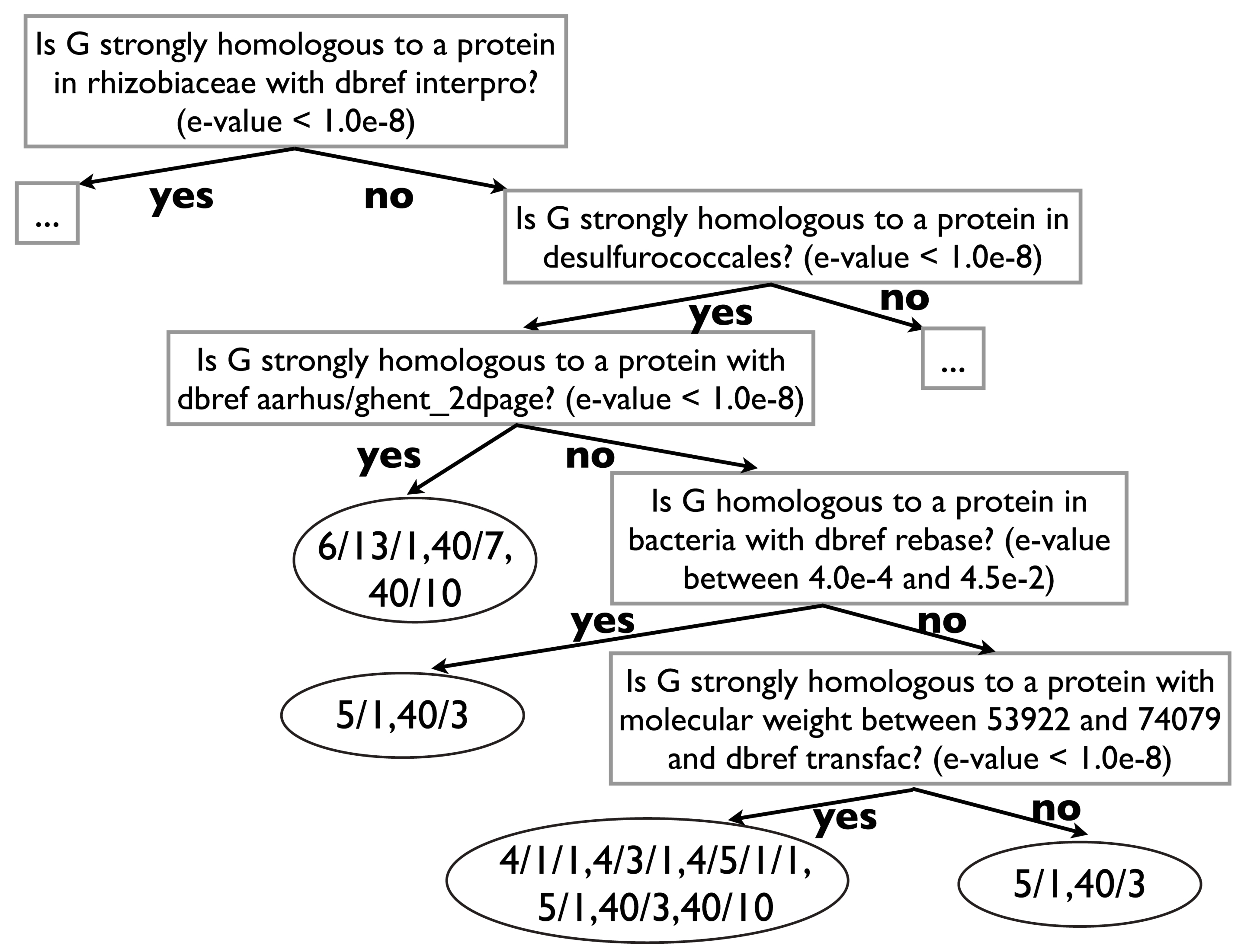
Interpretable Models
Interpretable Models
Example: Palmer Pinguins Dataset

Example: In Case of a Missing Library
Example: Loading the Data
Example: Using a DecisionTree
Example: Training
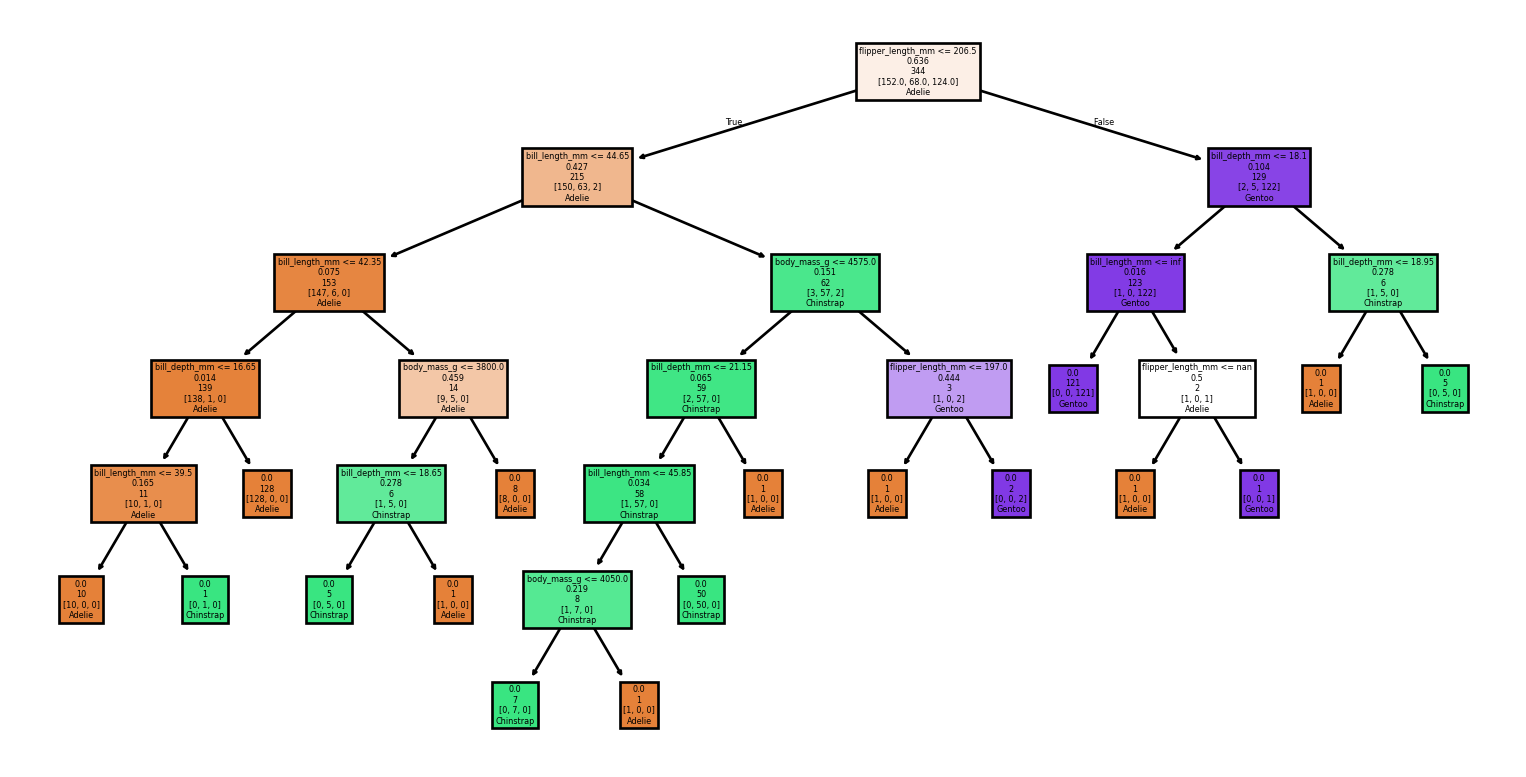
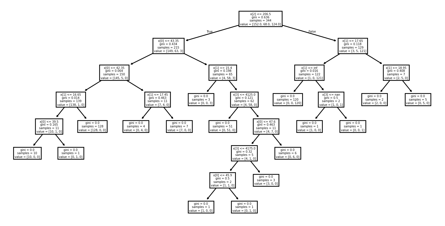
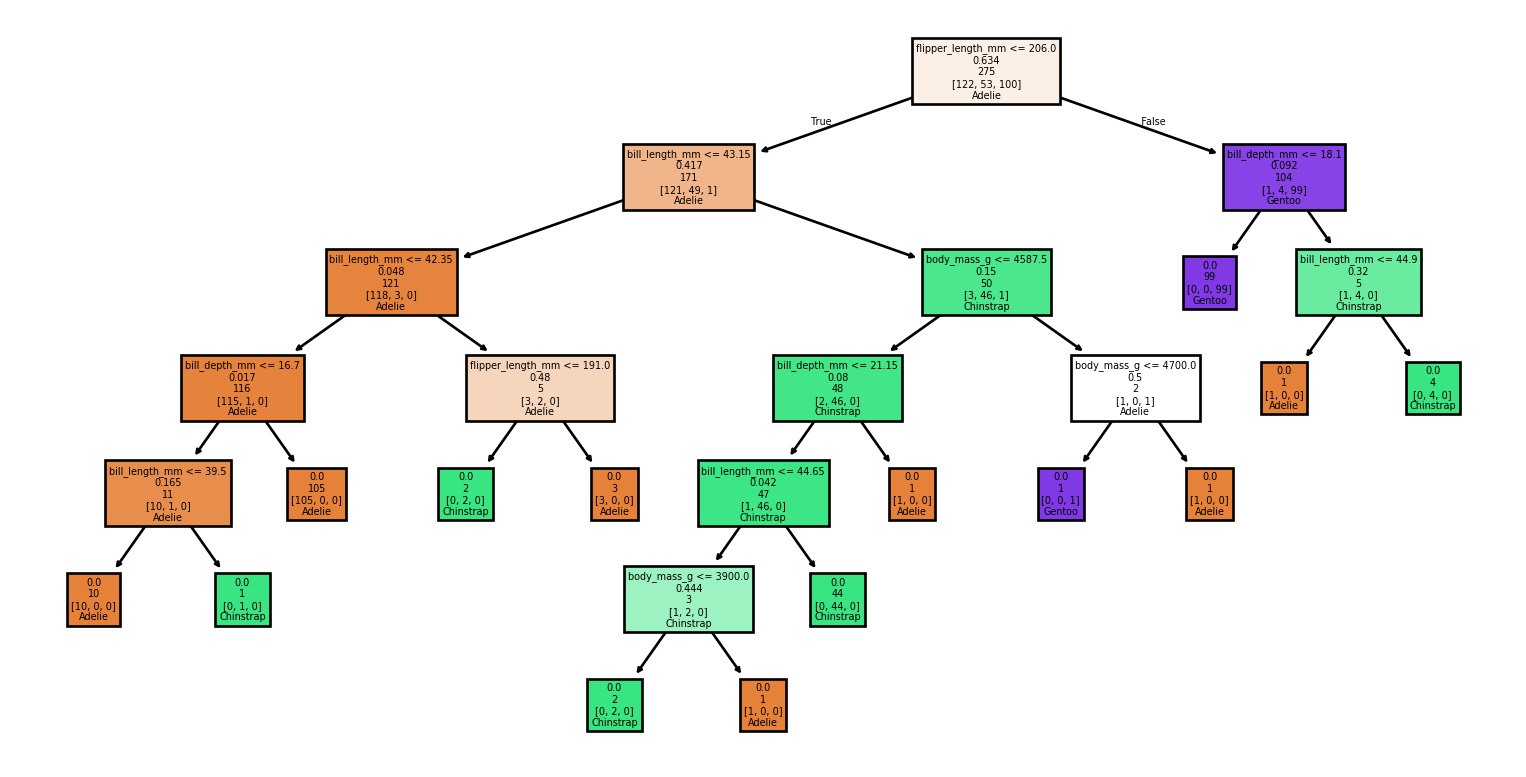
Example: Visualizing the tree (1/2)

Example: Visualizing the tree (2/2)
Example: Prediction
import pandas as pd

# Creating 2 test examples

columns_names = ['bill_length_mm', 'bill_depth_mm', 'flipper_length_mm', 'body_mass_g']
X_test = pd.DataFrame([[34.2, 17.9, 186.8, 2945.0], [51.0, 15.2, 223.7, 5560.0]], columns=columns_names)

# Prediction

y_test = clf.predict(X_test)

# Printing the predicted labels for our two examples

print(y_test)
['Adelie' 'Gentoo']Example: Complete
Example: Performance
from sklearn.metrics import classification_report, accuracy_score

# Make predictions

y_pred = clf.predict(X)

# Evaluate the model

accuracy = accuracy_score(y, y_pred)
report = classification_report(y, y_pred, target_names=target_names)

print(f'Accuracy: {accuracy:.2f}')
print('Classification Report:')
print(report)
Example: Performance
Accuracy: 1.00
Classification Report:
              precision    recall  f1-score   support

      Adelie       0.99      1.00      1.00       152
   Chinstrap       1.00      1.00      1.00        68
      Gentoo       1.00      0.99      1.00       124

    accuracy                           1.00       344
   macro avg       1.00      1.00      1.00       344
weighted avg       1.00      1.00      1.00       344
Example: Discussion
We have demonstrated a complete example:
- Loading the data
- Selecting a classifier
- Training the model
- Visualizing the model
- Making a prediction
Example: Wait a Minute!
from sklearn.metrics import classification_report, accuracy_score

# Make predictions

y_pred = clf.predict(X)

# Evaluate the model

accuracy = accuracy_score(y, y_pred)
report = classification_report(y, y_pred, target_names=target_names)

print(f'Accuracy: {accuracy:.2f}')
print('Classification Report:')
print(report)
Important
This example is misleading, or even flawed!
Example: Exploration
Example: Exploration
| species | island | bill_length_mm | bill_depth_mm | flipper_length_mm | body_mass_g | sex | year | |
|---|---|---|---|---|---|---|---|---|
| 0 | Adelie | Torgersen | 39.1 | 18.7 | 181.0 | 3750.0 | male | 2007 |
| 1 | Adelie | Torgersen | 39.5 | 17.4 | 186.0 | 3800.0 | female | 2007 |
| 2 | Adelie | Torgersen | 40.3 | 18.0 | 195.0 | 3250.0 | female | 2007 |
| 3 | Adelie | Torgersen | NaN | NaN | NaN | NaN | NaN | 2007 |
| 4 | Adelie | Torgersen | 36.7 | 19.3 | 193.0 | 3450.0 | female | 2007 |
Example: Exploration
Example: Exploration
| bill_length_mm | bill_depth_mm | flipper_length_mm | body_mass_g | year | |
|---|---|---|---|---|---|
| count | 342.000000 | 342.000000 | 342.000000 | 342.000000 | 344.000000 |
| mean | 43.921930 | 17.151170 | 200.915205 | 4201.754386 | 2008.029070 |
| std | 5.459584 | 1.974793 | 14.061714 | 801.954536 | 0.818356 |
| min | 32.100000 | 13.100000 | 172.000000 | 2700.000000 | 2007.000000 |
| 25% | 39.225000 | 15.600000 | 190.000000 | 3550.000000 | 2007.000000 |
| 50% | 44.450000 | 17.300000 | 197.000000 | 4050.000000 | 2008.000000 |
| 75% | 48.500000 | 18.700000 | 213.000000 | 4750.000000 | 2009.000000 |
| max | 59.600000 | 21.500000 | 231.000000 | 6300.000000 | 2009.000000 |
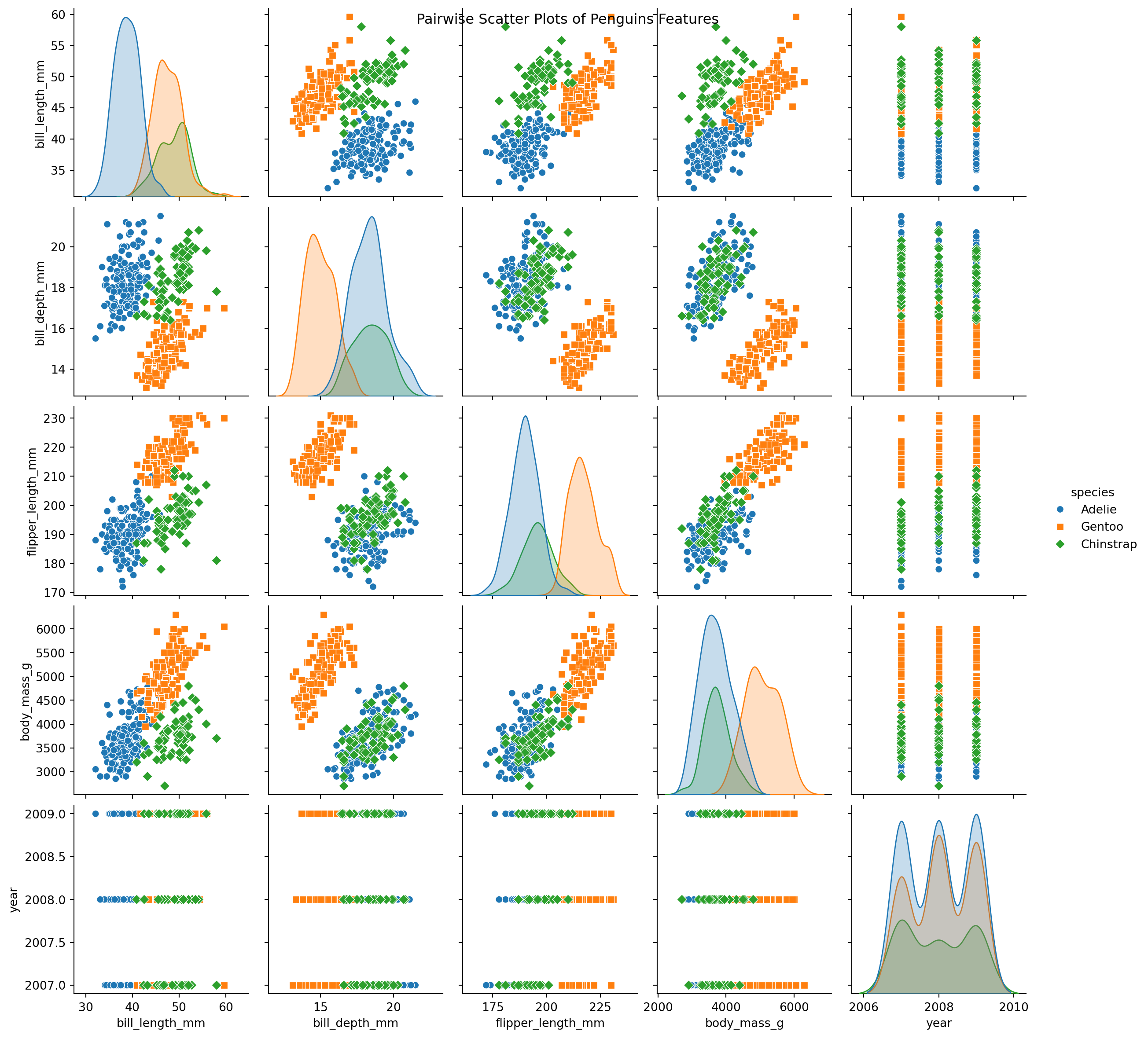
Example: Using Seaborn
Example: Using Seaborn
Example: Training and Test Set
Example: Creating a New Classifier
Example: Training the New Classifier
Example: Visualizing the Tree
Example: Making Predictions
Example: Measuring the Performance
Example: Measuring the Performance
Accuracy: 0.94
Classification Report:
              precision    recall  f1-score   support

      Adelie       0.96      0.90      0.93        30
   Chinstrap       0.94      1.00      0.97        15
      Gentoo       0.92      0.96      0.94        24

    accuracy                           0.94        69
   macro avg       0.94      0.95      0.95        69
weighted avg       0.94      0.94      0.94        69
Summary
- We introduced relevant terminology.
- Next, we will explore a complete example using scikit-learn.
- We performed a simple exploration of our data.
- Finally, we recognized the necessity of an independent test set to accurately measure performance.
Prologue
Further readings (1/3)
- The Hundred-Page Machine Learning Book (Burkov 2019) is a succinct and focused textbook that can feasibly be read in one week, making it an excellent introductory resource.
- Available under a “read first, buy later” model, allowing readers to evaluate its content before purchasing.
- Its author, Andriy Burkov, received his Ph.D. in AI from Université Laval.
Further readings (2/3)

- Hands-on Machine Learning with Scikit-Learn, Keras, and TensorFlow (Géron 2022) provides practical examples and leverages production-ready Python frameworks.
- Comprehensive coverage includes not only the models but also libraries for hyperparameter tuning, data preprocessing, and visualization.
- Code examples and solutions to exercises available as Jupyter Notebooks on GitHub.
- Aurélien Géron is a former YouTube Product Manager, who lead video classification for Search & Discovery.
Further readings (3/3)
- Mathematics for Machine Learning (Deisenroth, Faisal, and Ong 2020) aims to provide the necessary mathematical skills to read machine learning books.
- PDF of the book
- “This book provides great coverage of all the basic mathematical concepts for machine learning. I’m looking forward to sharing it with students, colleagues, and anyone interested in building a solid understanding of the fundamentals.” Joelle Pineau, McGill University and Facebook
Next Lecture
- Detailed presentation of decision trees
Appendix: Iris
Example: iris data set

Example: loading the Data
Example: Using a DecisionTree
Example: Training
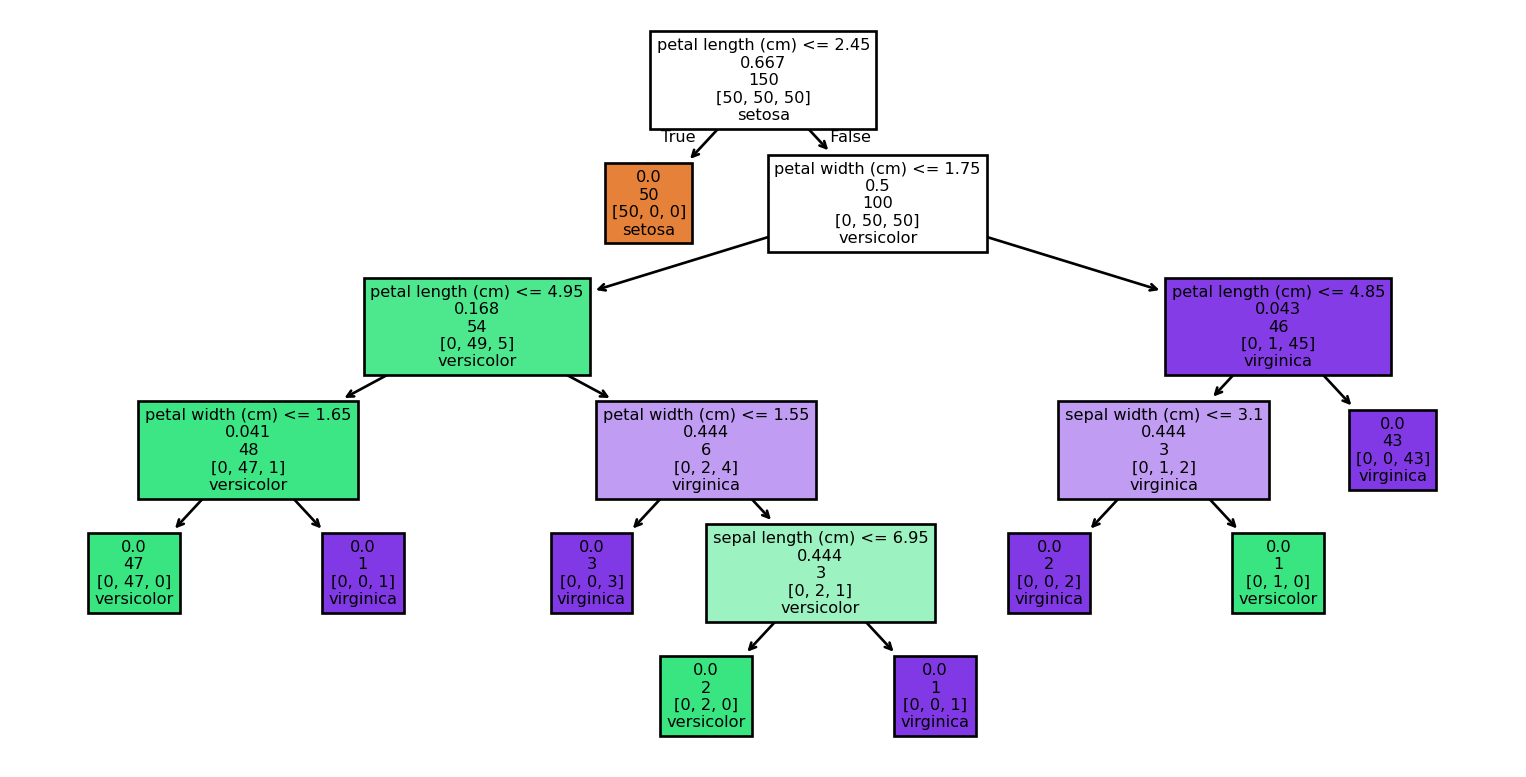
Example: Visualizing the tree (1/2)
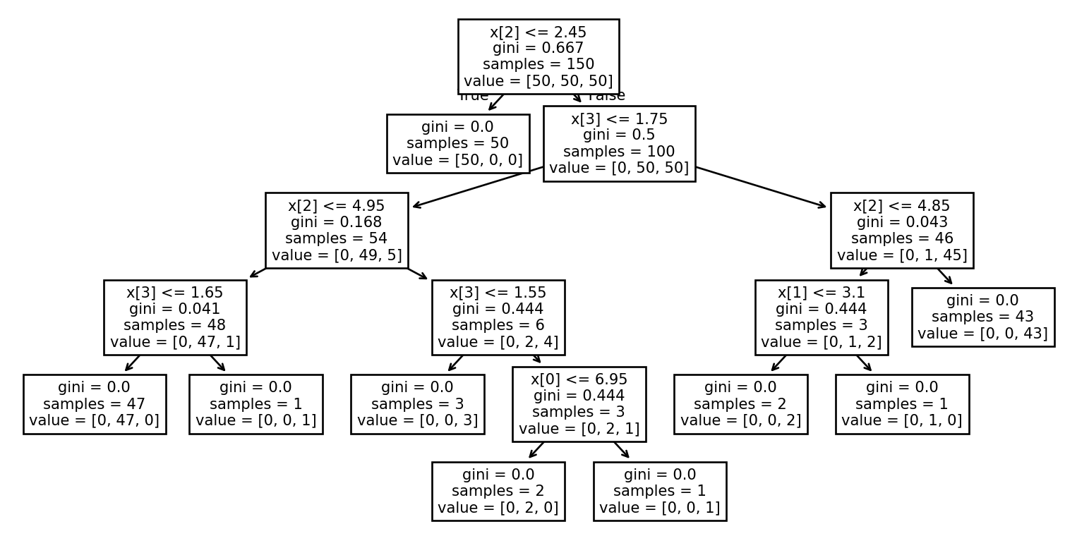
Example: Visualizing the tree (2/2)
Example: Prediction
# Creating 2 test examples
# 'sepal length (cm)', 'sepal width (cm)', 'petal length (cm)', 'petal width (cm)'

X_test = [[5.1, 3.5, 1.4, 0.2],[6.7, 3.0, 5.2, 2.3]]

# Prediction

y_test = clf.predict(X_test)

# Printing the predicted labels for our two examples

print(iris.target_names[y_test])
['setosa' 'virginica']Example: Complete

Example: Performance
from sklearn.metrics import classification_report, accuracy_score

# Make predictions

y_pred = clf.predict(X)

# Evaluate the model

accuracy = accuracy_score(y, y_pred)
report = classification_report(y, y_pred, target_names=iris.target_names)

print(f'Accuracy: {accuracy:.2f}')
print('Classification Report:')
print(report)Example: Performance
Accuracy: 1.00
Classification Report:
              precision    recall  f1-score   support

      setosa       1.00      1.00      1.00        50
  versicolor       1.00      1.00      1.00        50
   virginica       1.00      1.00      1.00        50

    accuracy                           1.00       150
   macro avg       1.00      1.00      1.00       150
weighted avg       1.00      1.00      1.00       150
Example: Discussion
We have demonstrated a complete example:
- Loading the data
- Selecting a classifier
- Training the model
- Visualizing the model
- Making a prediction
Example: Take 2
from sklearn.metrics import classification_report, accuracy_score

# Make predictions

y_pred = clf.predict(X)

# Evaluate the model

accuracy = accuracy_score(y, y_pred)
report = classification_report(y, y_pred, target_names=iris.target_names)

print(f'Accuracy: {accuracy:.2f}')
print('Classification Report:')
print(report)
Important
This example is misleading, or even flawed!
Example: Exploration
Dataset Description:
.. _iris_dataset:

Iris plants dataset
--------------------

**Data Set Characteristics:**

:Number of Instances: 150 (50 in each of three classes)
:Number of Attributes: 4 numeric, predictive attributes and the class
:Attribute Information:
    - sepal length in cm
    - sepal width in cm
    - petal length in cm
    - petal width in cm
    - class:
            - Iris-Setosa
            - Iris-Versicolour
            - Iris-Virginica

:Summary Statistics:

============== ==== ==== ======= ===== ====================
                Min  Max   Mean    SD   Class Correlation
============== ==== ==== ======= ===== ====================
sepal length:   4.3  7.9   5.84   0.83    0.7826
sepal width:    2.0  4.4   3.05   0.43   -0.4194
petal length:   1.0  6.9   3.76   1.76    0.9490  (high!)
petal width:    0.1  2.5   1.20   0.76    0.9565  (high!)
============== ==== ==== ======= ===== ====================

:Missing Attribute Values: None
:Class Distribution: 33.3% for each of 3 classes.
:Creator: R.A. Fisher
:Donor: Michael Marshall (MARSHALL%PLU@io.arc.nasa.gov)
:Date: July, 1988

The famous Iris database, first used by Sir R.A. Fisher. The dataset is taken
from Fisher's paper. Note that it's the same as in R, but not as in the UCI
Machine Learning Repository, which has two wrong data points.

This is perhaps the best known database to be found in the
pattern recognition literature.  Fisher's paper is a classic in the field and
is referenced frequently to this day.  (See Duda & Hart, for example.)  The
data set contains 3 classes of 50 instances each, where each class refers to a
type of iris plant.  One class is linearly separable from the other 2; the
latter are NOT linearly separable from each other.

.. dropdown:: References

  - Fisher, R.A. "The use of multiple measurements in taxonomic problems"
    Annual Eugenics, 7, Part II, 179-188 (1936); also in "Contributions to
    Mathematical Statistics" (John Wiley, NY, 1950).
  - Duda, R.O., & Hart, P.E. (1973) Pattern Classification and Scene Analysis.
    (Q327.D83) John Wiley & Sons.  ISBN 0-471-22361-1.  See page 218.
  - Dasarathy, B.V. (1980) "Nosing Around the Neighborhood: A New System
    Structure and Classification Rule for Recognition in Partially Exposed
    Environments".  IEEE Transactions on Pattern Analysis and Machine
    Intelligence, Vol. PAMI-2, No. 1, 67-71.
  - Gates, G.W. (1972) "The Reduced Nearest Neighbor Rule".  IEEE Transactions
    on Information Theory, May 1972, 431-433.
  - See also: 1988 MLC Proceedings, 54-64.  Cheeseman et al"s AUTOCLASS II
    conceptual clustering system finds 3 classes in the data.
  - Many, many more ...
Example: Exploration
Feature Names: ['sepal length (cm)', 'sepal width (cm)', 'petal length (cm)', 'petal width (cm)']Example: Using Pandas (continued)
Example: Using Pandas (continued)
Example: Using Pandas (continued)
sepal length (cm) sepal width (cm) petal length (cm) \
count 150.000000 150.000000 150.000000
mean 5.843333 3.057333 3.758000
std 0.828066 0.435866 1.765298
min 4.300000 2.000000 1.000000
25% 5.100000 2.800000 1.600000
50% 5.800000 3.000000 4.350000
75% 6.400000 3.300000 5.100000
max 7.900000 4.400000 6.900000
petal width (cm) species
count 150.000000 150.000000
mean 1.199333 1.000000
std 0.762238 0.819232
min 0.100000 0.000000
25% 0.300000 0.000000
50% 1.300000 1.000000
75% 1.800000 2.000000
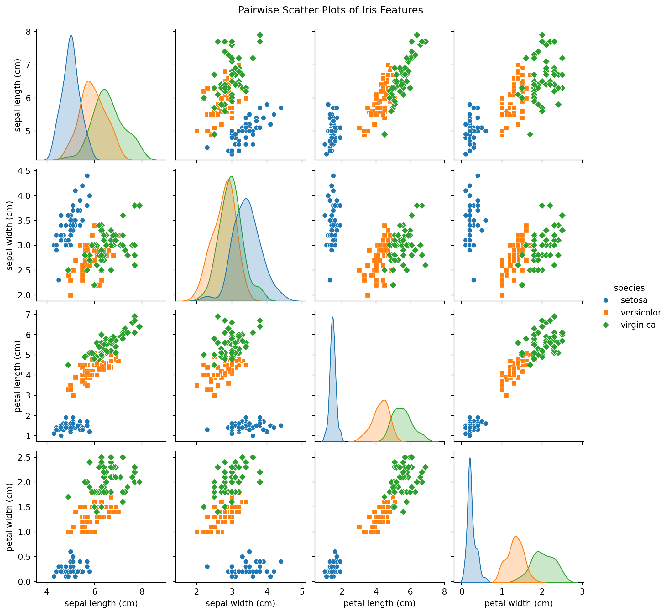
max 2.500000 2.000000 Example: Using Seaborn
Example: Using Seaborn
Example: Training and test set
Example: Creating a new classifier
Example: Training the new classifier
Example: Making predictions
Example: measuring the performance
from sklearn.metrics import classification_report, accuracy_score
# Make predictions

# Evaluate the model
accuracy = accuracy_score(y_test, y_pred)
report = classification_report(y_test, y_pred, target_names=iris.target_names)

print(f'Accuracy: {accuracy:.2f}')
print('Classification Report:')
print(report)Example: measuring the performance
Accuracy: 0.90
Classification Report:
              precision    recall  f1-score   support

      setosa       1.00      1.00      1.00         7
  versicolor       0.91      0.83      0.87        12
   virginica       0.83      0.91      0.87        11

    accuracy                           0.90        30
   macro avg       0.91      0.91      0.91        30
weighted avg       0.90      0.90      0.90        30
References
Marcel Turcotte
School of Electrical Engineering and Computer Science (EECS)
University of Ottawa