Decision Trees

CSI 5180 - Machine Learning for Bioinformatics

Marcel Turcotte

Version: Jan 29, 2025 10:40

Preamble

Quote of the Day

Summary

This lecture explores decision trees, emphasizing their interpretability as a key advantage. Decision trees adeptly handle diverse feature types, facilitating seamless integration of heterogeneous data. Their performance is notably enhanced within ensemble learning frameworks, demonstrating robust predictive accuracy.

General objective:

• Explain what decision trees are, how they are built, and how they can be used to classify data.

Learning Outcomes

• Describe the basic structure of a decision tree and how it processes data.
• Explain the concepts of impurity, overfitting, and regularization in the context of decision trees.
• Recognize how decision trees can be combined in ensemble methods (e.g., random forests) for improved stability and accuracy.
• Demonstrate the application of decision trees to real-world bioinformatics tasks (e.g., single-cell classification).

Decision Trees

Rationale

• Understanding foundational learning algorithms is crucial for contextualizing advanced topics.

• Many algorithms leverage gradient-based optimization, making familiarity with a diverse range of algorithms essential.

• Fundamental concepts, including generalization, underfitting, overfitting, regularization, and ensemble learning, will be explored in greater detail in subsequent discussions.

Rationale

• Decision Trees are algorithms employed in supervised learning paradigms.
• Applications:
  • Classification: Assigns instances to predefined classes based on input features (\(y_i\) is a class).
  • Regression: Predicts continuous output values (\(y_i\) is a real value).

Rationale

• Essential components of Random Forest algorithms, particularly effective with small datasets.
• Produce models that are easily interpretable by humans.

Rationale

• Handle both categorical and continuous features, with certain implementations accommodating missing data.
• As non-parametric models, they do not assume any specific data distribution, offering flexibility across diverse data types and distributions.
• Capable of modeling complex non-linear relationships between features and target variables without requiring explicit data transformations.

Interpretable Models

Schietgat et al. (2010)

Interpretable Models

Schietgat et al. (2010)

What is a Decision Tree?

• A decision tree is a hierarchical structure represented as a directed acyclic graph, utilized for classification and regression tasks.
• Each internal node conducts a binary test on a specific feature (\(j\)), such as determining if the expression level of a gene in a sample exceeds a defined threshold.
• The leaves function as decision nodes.
• The tree’s structure is inferred (learnt) from the training data.

What is a Decision Tree?

• Decision trees can extend beyond binary splits, as exemplified by algorithms like ID3, which accommodate nodes with multiple children.

Classifying New Instances (Inference)

• Begin at the root node of the decision tree. Proceed by answering a sequence of binary questions until a leaf node is reached. The label associated with this leaf denotes the classification of the instance.
• Alternatively, some algorithms may store a probability distribution at the leaf, representing the fraction of training samples corresponding to each class \(k\), across all possible classes \(k\).

Decision Boundary

Palmer Pinguins Dataset

# Loading our dataset

try:
  from palmerpenguins import load_penguins
except:
  ! pip install palmerpenguins
  from palmerpenguins import load_penguins

penguins = load_penguins()

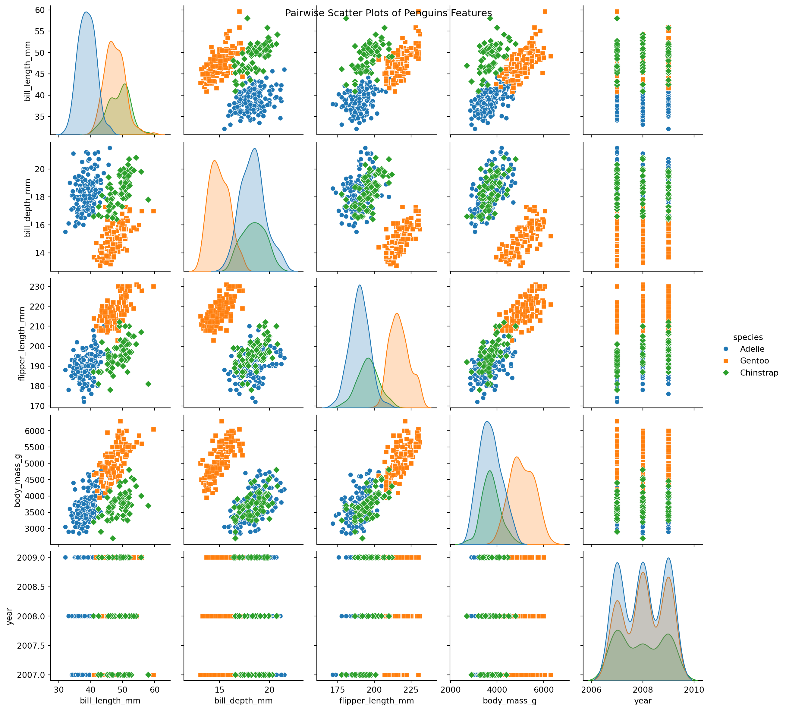
# Pairplot using seaborn

import matplotlib.pyplot as plt
import seaborn as sns

sns.pairplot(penguins, hue='species', markers=["o", "s", "D"])
plt.suptitle("Pairwise Scatter Plots of Penguins Features")
plt.show()

Palmer Pinguins Dataset

Binary Classification Problem

• Several scatter plots reveal a distinct clustering of Gentoo instances.
• To illustrate our next exemple, we propose a binary classification model: Gentoo versus non-Gentoo.
• Our analysis will concentrate on two key features: body mass and bill depth.

Definition

A decision boundary is a “boundary” that partitions the underlying feature space into regions corresponding to different class labels.

The term boundary will be clarified over the next slides.

Decision Boundary

The decision boundary between these attributes can be represented as a line.

# Import necessary libraries
import numpy as np
from sklearn.linear_model import LogisticRegression
from sklearn.model_selection import train_test_split

try:
  from palmerpenguins import load_penguins
except:
  ! pip install palmerpenguins
  from palmerpenguins import load_penguins

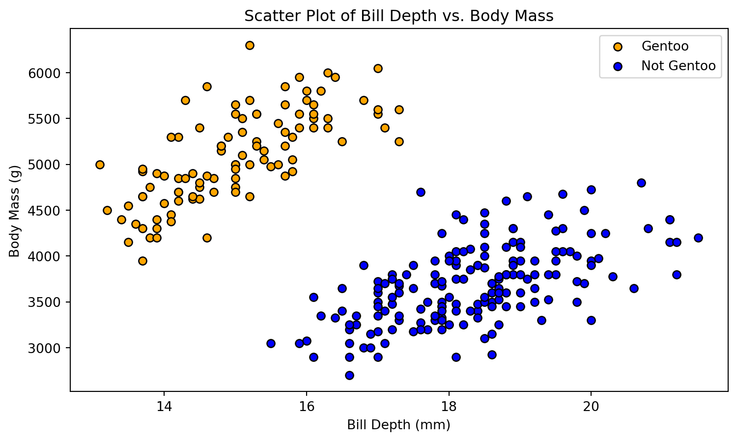
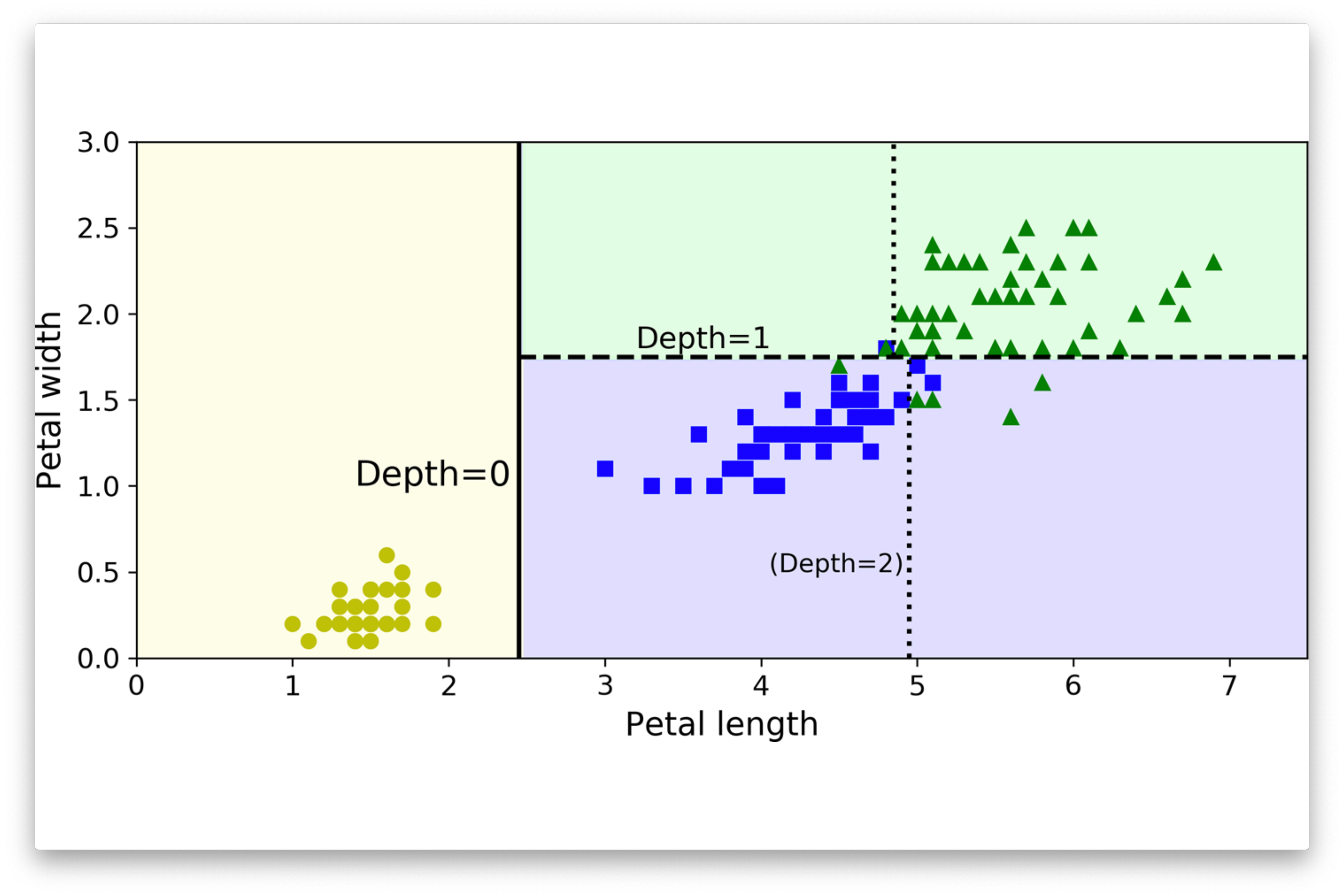
# Load the Palmer Penguins dataset
df = load_penguins()

# Preserve only the necessary features: 'bill_depth_mm' and 'body_mass_g'
features = ['bill_depth_mm', 'body_mass_g']
df = df[features + ['species']]

# Drop rows with missing values
df.dropna(inplace=True)

# Create a binary problem: 'Gentoo' vs 'Not Gentoo'
df['species_binary'] = df['species'].apply(lambda x: 1 if x == 'Gentoo' else 0)

# Define feature matrix X and target vector y
X = df[features].values
y = df['species_binary'].values

# Split the data into training and testing sets
X_train, X_test, y_train, y_test = train_test_split(X, y, test_size=0.2, random_state=42)

# Function to plot initial scatter of data
def plot_scatter(X, y):
    plt.figure(figsize=(9, 5))
    plt.scatter(X[y == 1, 0], X[y == 1, 1], color='orange', edgecolors='k', marker='o', label='Gentoo')
    plt.scatter(X[y == 0, 0], X[y == 0, 1], color='blue', edgecolors='k', marker='o', label='Not Gentoo')
    plt.xlabel('Bill Depth (mm)')
    plt.ylabel('Body Mass (g)')
    plt.title('Scatter Plot of Bill Depth vs. Body Mass')
    plt.legend()
    plt.show()
    
# Plot the initial scatter plot
plot_scatter(X_train, y_train)

Decision Boundary

Decision Boundary

The decision boundary between these attributes can be represented as a line.

# Train a logistic regression model
model = LogisticRegression()
model.fit(X_train, y_train)

# Function to plot decision boundary
def plot_decision_boundary(X, y, model):
    x_min, x_max = X[:, 0].min() - 1, X[:, 0].max() + 1
    y_min, y_max = X[:, 1].min() - 1, X[:, 1].max() + 1
    xx, yy = np.meshgrid(np.arange(x_min, x_max, 0.1),
                         np.arange(y_min, y_max, 0.1))
    Z = model.predict(np.c_[xx.ravel(), yy.ravel()])
    Z = Z.reshape(xx.shape)
    
    plt.figure(figsize=(9, 5))
    plt.contourf(xx, yy, Z, alpha=0.3, cmap='RdYlBu')
    plt.scatter(X[y == 1, 0], X[y == 1, 1], color='orange', edgecolors='k', marker='o', label='Gentoo')
    plt.scatter(X[y == 0, 0], X[y == 0, 1], color='blue', edgecolors='k', marker='o', label='Not Gentoo')
    plt.xlabel('Bill Depth (mm)')
    plt.ylabel('Body Mass (g)')
    plt.title('Logistic Regression Decision Boundary')
    plt.legend()
    plt.show()

# Plot the decision boundary on the training set
plot_decision_boundary(X_train, y_train, model)

Decision Boundary

Definition

We say that the data is linearly separable when two classes of data can be perfectly separated by a single linear boundary, such as a line in two-dimensional space or a hyperplane in higher dimensions.

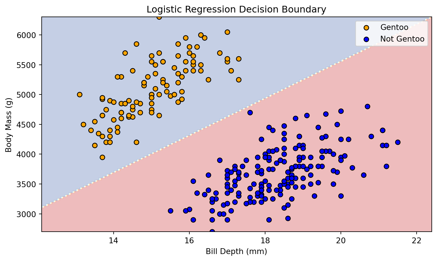
Simple Decision Doundary

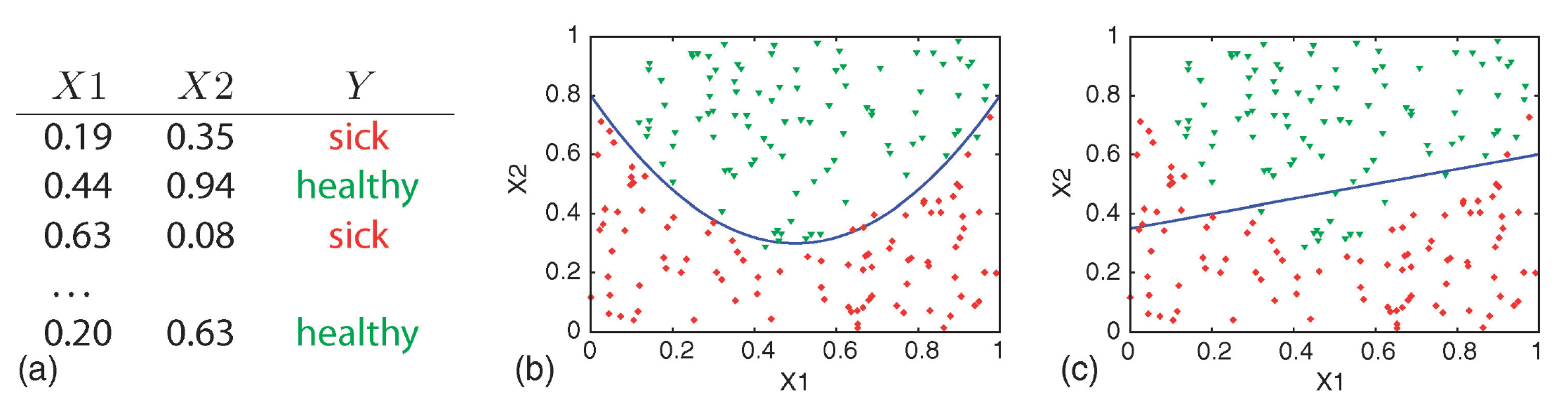
(a) training data, (b) quadratic curve, and (c) linear function.

Attribution: (Geurts, Irrthum, and Wehenkel 2009)

The table on the left presents training data for a hypothetical binary classification task in a medical context, where the two attributes, \(X_1\) and \(X_2\), are used to predict the target variable, \(y\), which can take on two values: sick and healthy. You can imagine that \(X_1\) and \(X_2\) are measurements, such as blood pressure and heart rate or cholesterol and glucose levels.

Logistic regression (c) employs a linear decision boundary. In this specific example, the decision boundary is represented by a straight line. Employing logistic regression for this problem results in several classification errors: red dots above the line, which should be classified as ‘sick’, are incorrectly predicted as ‘healthy’. Conversely, green dots below the line, which should be classified as ‘healthy’, are incorrectly predicted as ‘sick’.

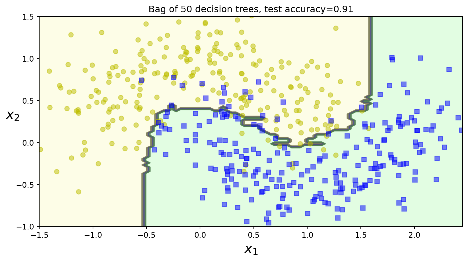
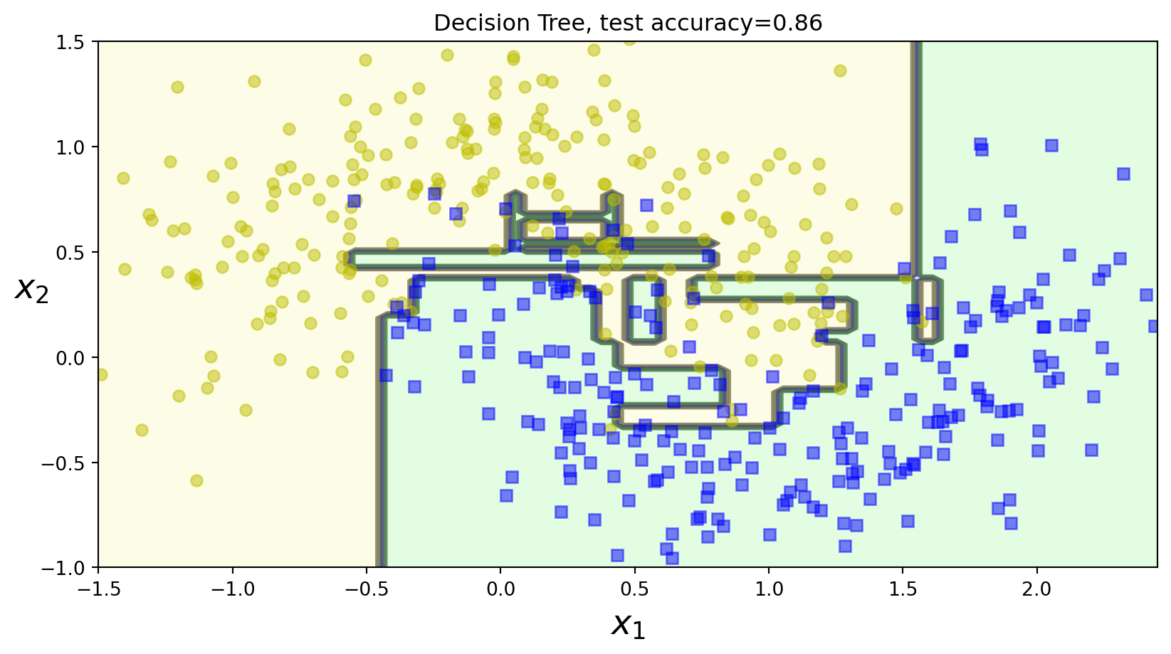
Complex Decision Boundary

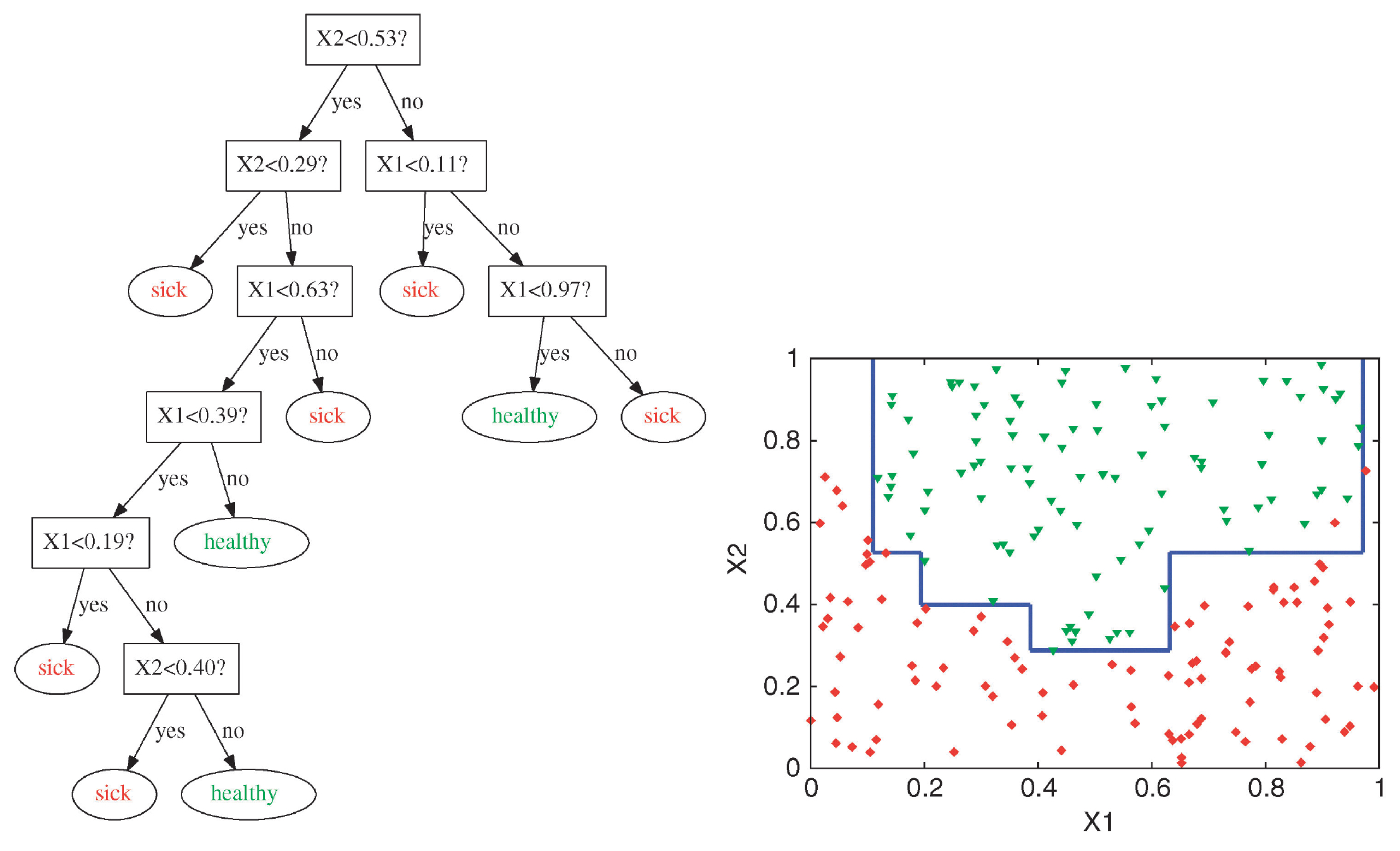
Decision trees are capable of generating irregular and non-linear decision boundaries.

Attribution: ibidem.

Make sure to understand the relationships between the eight decision rules delineated in the decision tree and the nine line segments represented in the scatter plot.

Decision Boundary

import numpy as np
import matplotlib.pyplot as plt
from mpl_toolkits.mplot3d import Axes3D

# Function to generate points
def generate_points_above_below_plane(num_points=100):
    # Define the plane z = ax + by + c
    a, b, c = 1, 1, 0  # Plane coefficients

    # Generate random points
    x1 = np.random.uniform(-10, 10, num_points)
    x2 = np.random.uniform(-10, 10, num_points)

    y1 = np.random.uniform(-10, 10, num_points)
    y2 = np.random.uniform(-10, 10, num_points)

    # Points above the plane
    z_above = a * x1 + b * y1 + c + np.random.normal(20, 2, num_points)

    # Points below the plane
    z_below = a * x2 + b * y2 + c - np.random.normal(20, 2, num_points)

    # Stack the points into arrays
    points_above = np.vstack((x1, y1, z_above)).T
    points_below = np.vstack((x2, y2, z_below)).T

    return points_above, points_below

# Generate points
points_above, points_below = generate_points_above_below_plane()

# Visualization
fig = plt.figure(figsize=(8,6))
ax = fig.add_subplot(111, projection='3d')

# Plot points above the plane
ax.scatter(points_above[:, 0], points_above[:, 1], points_above[:, 2], c='r', label='Positive')

# Plot points below the plane
ax.scatter(points_below[:, 0], points_below[:, 1], points_below[:, 2], c='b', label='Negative')

# Plot the plane itself for reference
xx, yy = np.meshgrid(range(-10, 11), range(-10, 11))
zz = 1 * xx + 1 * yy + 0
ax.plot_surface(xx, yy, zz, alpha=0.2, color='gray')

# Set labels
ax.set_xlabel('X1')
ax.set_ylabel('X2')
ax.set_zlabel('X3')

ax.view_init(elev=-90, azim=90)

# Set title and legend
ax.set_title('Binary classification')
ax.legend()

# Show plot
plt.show()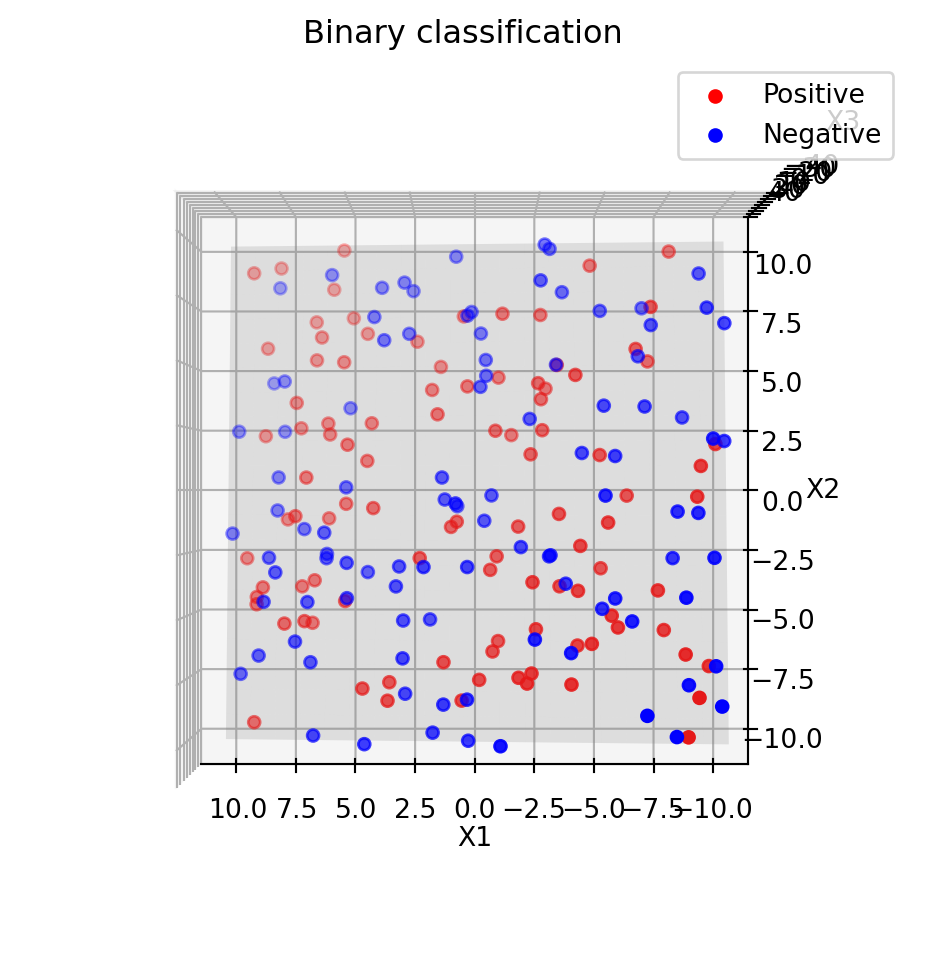

Separating the data using these two attributes, \(x1\) and \(x2\), is infeasible.

Decision Boundary

import numpy as np
import matplotlib.pyplot as plt
from mpl_toolkits.mplot3d import Axes3D

# Function to generate points
def generate_points_above_below_plane(num_points=100):
    # Define the plane z = ax + by + c
    a, b, c = 1, 1, 0  # Plane coefficients

    # Generate random points
    x1 = np.random.uniform(-10, 10, num_points)
    x2 = np.random.uniform(-10, 10, num_points)

    y1 = np.random.uniform(-10, 10, num_points)
    y2 = np.random.uniform(-10, 10, num_points)

    # Points above the plane
    z_above = a * x1 + b * y1 + c + np.random.normal(20, 2, num_points)

    # Points below the plane
    z_below = a * x2 + b * y2 + c - np.random.normal(20, 2, num_points)

    # Stack the points into arrays
    points_above = np.vstack((x1, y1, z_above)).T
    points_below = np.vstack((x2, y2, z_below)).T

    return points_above, points_below

# Generate points
points_above, points_below = generate_points_above_below_plane()

# Visualization
fig = plt.figure(figsize=(10,8))
ax = fig.add_subplot(111, projection='3d')

# Plot points above the plane
ax.scatter(points_above[:, 0], points_above[:, 1], points_above[:, 2], c='r', label='Above the plane (positive)')

# Plot points below the plane
ax.scatter(points_below[:, 0], points_below[:, 1], points_below[:, 2], c='b', label='Below the plane (negative)')

# Plot the plane itself for reference
xx, yy = np.meshgrid(range(-10, 11), range(-10, 11))
zz = 1 * xx + 1 * yy + 0
ax.plot_surface(xx, yy, zz, alpha=0.2, color='gray')

# Set labels
ax.set_xlabel('X1')
ax.set_ylabel('X2')
ax.set_zlabel('X3')

ax.view_init(elev=10, azim=-35)

# Set title and legend
ax.set_title('Binary classification, 3 attributes, linear decision boundary')
ax.legend()

# Show plot
plt.show()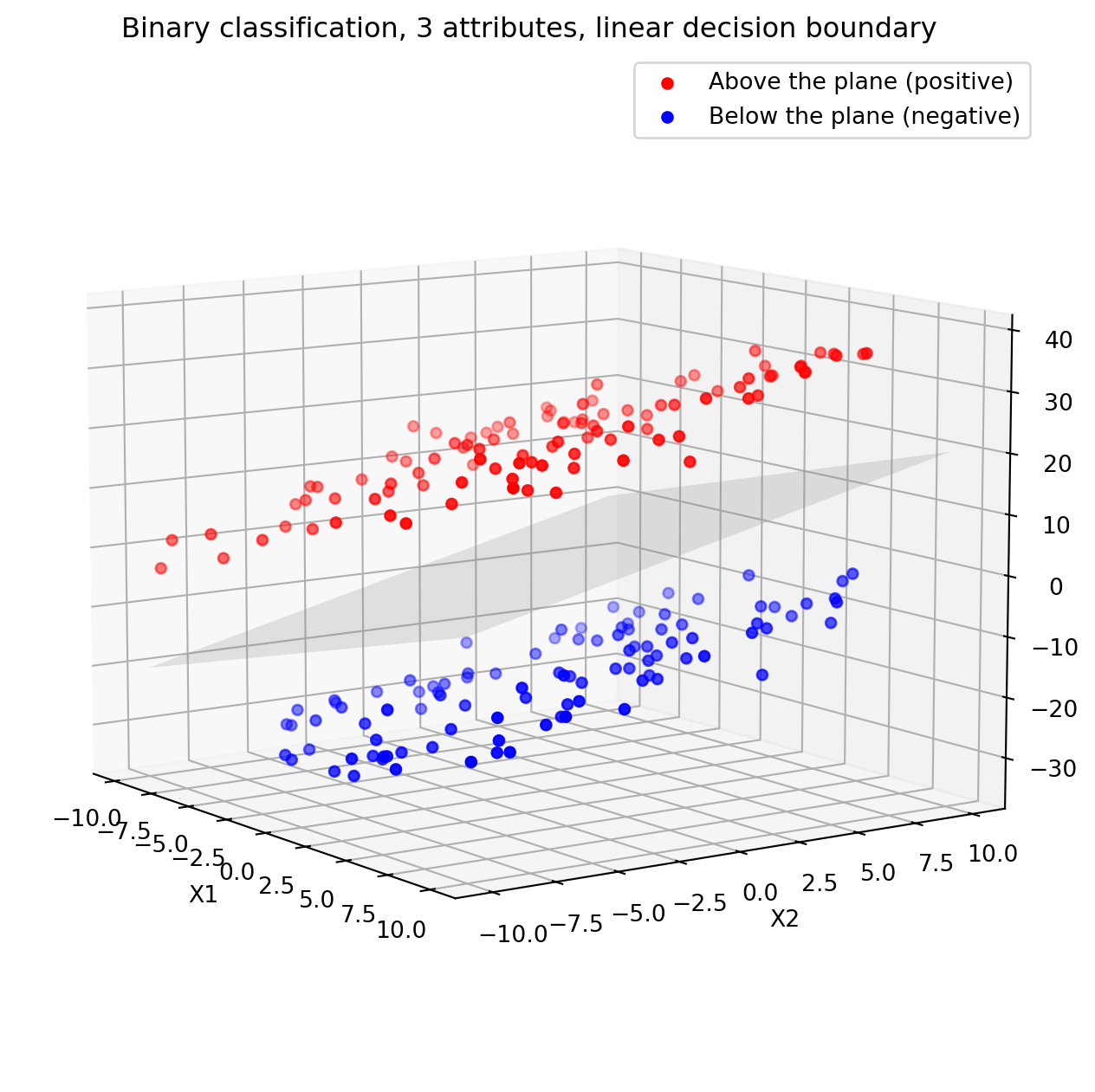

Adding attributes can help making the data (linearly) separable.

Definition (revised)

A decision boundary is a hypersurface that partitions the underlying feature space into regions corresponding to different class labels.

Construction

Constructing a Decision Tree

• How to construct (learnt) a decision tree?

• Are there some trees that are “better” than others?

• Is it feasible to construct an optimal decision tree with computational efficiency?

(Hyafil and Rivest 1976)

Optimality

• Let \(X = \{x_1, \ldots, x_n\}\) be a finite set of objects.
• Let \(\mathcal{T} = \{T_1, \ldots, T_t\}\) be a finite set of tests.
• For each object and test, we have:
  • \(T_i(x_j)\) is either true or false.
• An optimal tree is one that completely identifies all the objects in \(X\) and \(|T|\) is minimum.

(Hyafil and Rivest 1976)

Constructing a Decision Tree

• Iterative development: Initiate with an empty tree. Progressively introduce nodes, each informed by the training dataset, continuing until the dataset is completely classified or alternative termination criteria, such as maximum tree depth, are met.

Constructing a Decision Tree

• Initial Node Construction:
  • To establish the root node, evaluate all available \(D\) features.
    • For each feature, assess various threshold values derived from the observed data within the training set.

Constructing a Decision Tree

• For a numerical feature, the algorithm considers all possible split points (thresholds) in the feature’s range.
• These split points are typically the midpoints between two consecutive, sorted unique values of the feature.

Constructing a Decision Tree

• For a categorical feature with \(k\) unique values, the algorithm considers all possible ways of splitting the categories into two groups.
• For instance, if the feature (tissue type) has values \(\{\mathrm{brain}, \mathrm{hearth}, \mathrm{liver}\}\), it might evaluate splits like \(\{\mathrm{brain}\}\) vs. \(\{\mathrm{hearth}, \mathrm{liver}\}\), \(\{\mathrm{liver}\}\) vs. \(\{\mathrm{brain}, \mathrm{hearth}\}\) , etc.

Evaluation

What defines a “good” data split?

• \(\{\mathrm{brain}\}\) vs. \(\{\mathrm{hearth}, \mathrm{liver}\}\) : \([20,15]\) and \([20,15]\).
• \(\{\mathrm{liver}\}\) vs. \(\{\mathrm{brain}, \mathrm{hearth}\}\) : \([40,0]\) and \([0,30]\).

Where \([20,15]\) indicates that the subgroup contains 20 examples of the ‘up-regulated’ class and 15 examples of the ‘down-regulated’ class in a hypothetical binary classification problem for gene expression.

Evaluation

• Heterogeneity (also referred to as impurity) and homogeneity are critical metrics for evaluating the composition of resulting data partitions.

• Optimally, each of these partitions should contain data entries from a single class to achieve maximum homogeneity.

• Entropy and the Gini index are two widely utilized metrics for assessing these characteristics.

Evalution

Objective function for sklearn.tree.DecisionTreeClassifier (CART):

\[ J(k,t_k) = \frac{m_{\text{left}}}{m} G_{\text{left}} + \frac{m_{\text{right}}}{m} G_{\text{right}} \]

• The cost of partitioning the data using feature \(k\) and threshold \(t_k\).

• \(m_{\text{left}}\) and \(m_{\text{right}}\) is the number of examples in the left and right subsets, respectively, and \(m\) is the number of examples before splitting the data.

• \(G_{\text{left}}\) and \(G_{\text{right}}\) is the impurity of the left and right subsets, respectively.

CART minimizes \(J\).

Gini Index

• Gini index (default)

\[ G_i = 1 - \sum_{k=1}^n p_{i,k}^2 \]

• \(p_{i,k}\) is the proportion of the examples from this class \(k\) in the node \(i\).

• What is the maximum value of the Gini index?

• The value of the Gini index is maximum when all the classes are equiprobable, i.e. the proportions are the same.

• For a binary classification, \(1 - \[\frac{1}{2}^2 + \frac{1}{2}^2] = 0.5\).

• For the general case, \(1 - n \times \frac{1}{n}^2 = 1 - \frac{1}{n}\), as \(n \to \infty\), the Gini index tends to 1.

Gini Index

Examples:

• \(1 - (0/100)^2 + (100/100)^2 = 0\) (pure)
• \(1 - (25/100)^2 + (75/100)^2 = 0.375\)
• \(1 - (50/100)^2 + (50/100)^2 = 0.5\)

Gini Index

def gini_index(p):
    """Calculate the Gini index."""
    return 1 - (p**2 + (1 - p)**2)

# Probability values for class 1
p_values = np.linspace(0, 1, 100)

# Calculate Gini index for each probability
gini_values = [gini_index(p) for p in p_values]

# Plot the Gini index
plt.figure(figsize=(8, 6))
plt.plot(p_values, gini_values, label='Gini Index', color='b')
plt.title('Gini Index for Binary Classification')
plt.xlabel('Probability of Class 1 (p)')
plt.ylabel('Gini Index')
plt.grid(True)
plt.legend()
plt.show()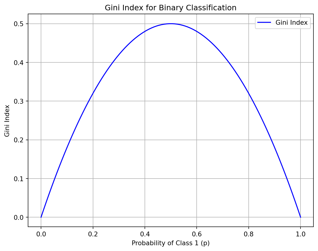

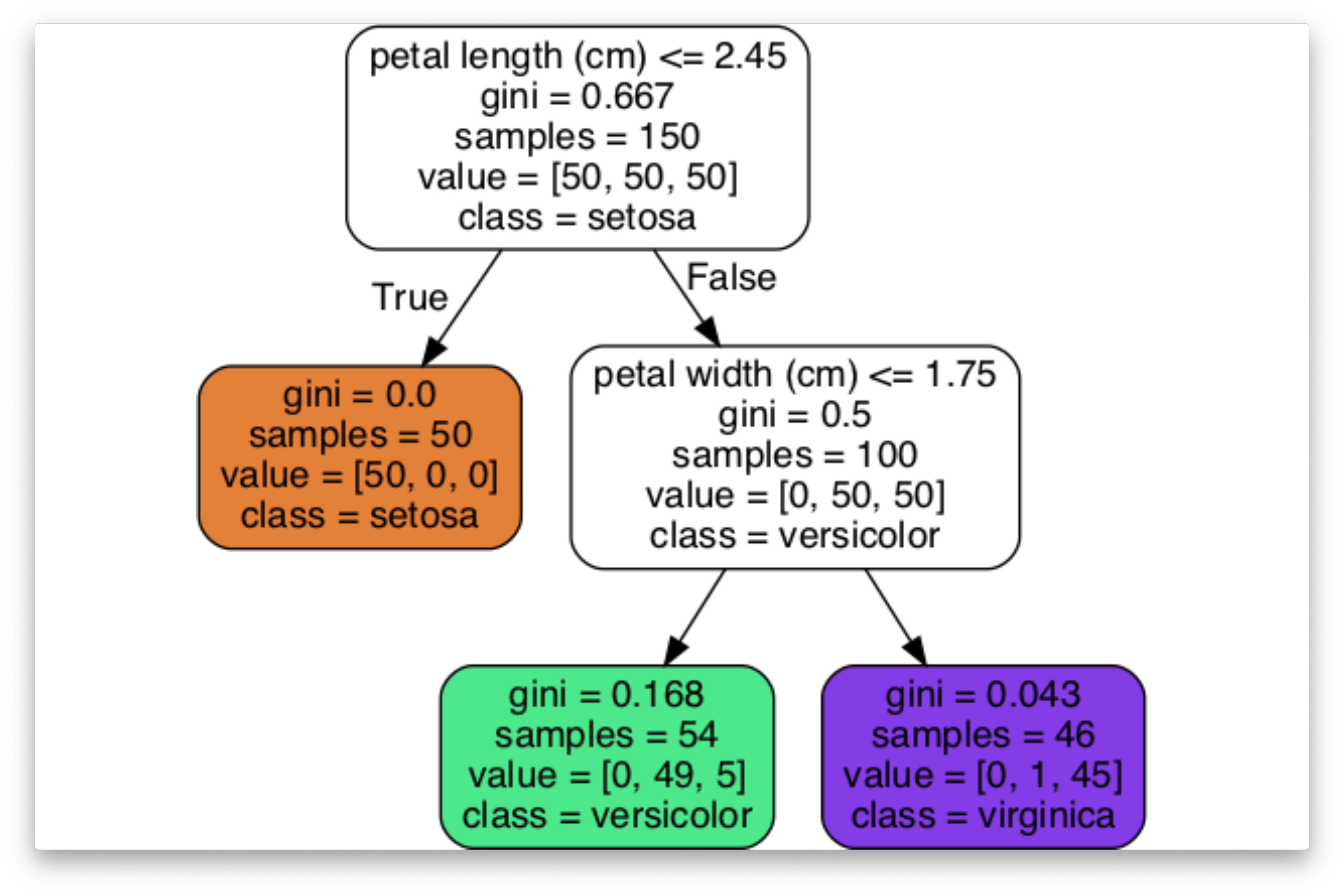
Iris Dataset

Attribution: (Géron 2019), Figures 6.1 and 6.2

Complete Example

Entropy

Entropy in information theory quantifies the uncertainty or unpredictability of a random variable’s possible outcomes. It measures the average amount of information produced by a stochastic source of data and is typically expressed in bits for binary systems. The entropy \(H\) of a discrete random variable \(X\) with possible outcomes \(\{x_1, x_2, \ldots, x_n\}\) and probability mass function \(P(X)\) is given by:

\[ H(X) = -\sum_{i=1}^n P(x_i) \log_2 P(x_i) \]

Entropy

Entropy is maximized when all outcomes are equally likely, in which case it equals the logarithm of the number of outcomes:

\[ H_{\text{max}} = \log_2(n) \]

Entropy

import numpy as np
import matplotlib.pyplot as plt

# Function to compute entropy
def entropy(p):
    if p == 0 or p == 1:
        return 0
    return -p * np.log2(p) - (1 - p) * np.log2(1 - p)

# Generate probabilities from 0 to 1
probabilities = np.linspace(0, 1, 1000)

# Compute entropy for each probability
entropies = [entropy(p) for p in probabilities]

# Plot the results
plt.figure(figsize=(10, 6))
plt.plot(probabilities, entropies, label='Entropy H(p)', color='blue')
plt.title('Entropy for a Single Variable with Two Outcomes')
plt.xlabel('Probability p')
plt.ylabel('Entropy H(p)')
plt.grid(True)
plt.legend()
plt.show()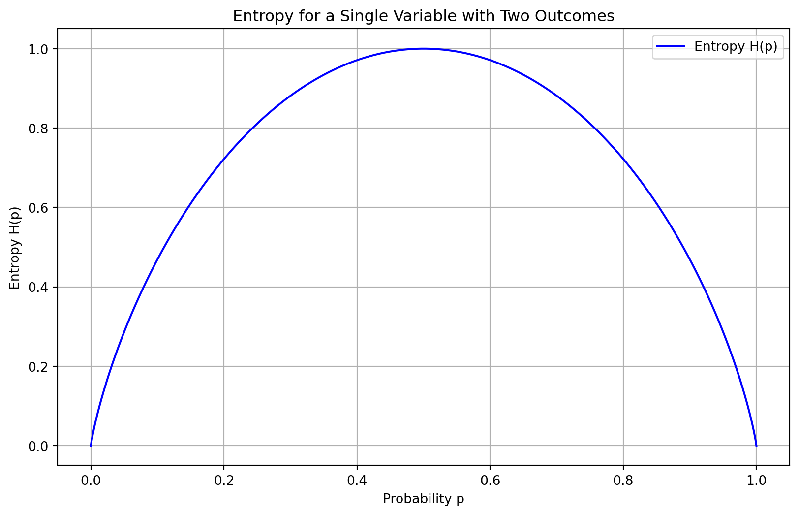

Entropy

• Entropy and Gini produce similar results:
  • sebastianraschka.com/faq/docs/decision-tree-binary.html

Stopping Criteria

• All the examples in a given node belong to the same class.
• Depth of the tree would exceed max_depth.
• Number of examples in the node is min_sample_split or less.
• None of the splits decreases impurity sufficiently (min_impurity_decrease).
• See documentation for other criteria.

Limitation

Limitations

• Possibly creates large trees
  • Challenge for interpretation
  • Overfitting
• Greedy algorithm, no guarantee to find the optimal tree. (Hyafil and Rivest 1976)
• Small changes to the data set produce vastly different trees

Large Trees

(Stiglic et al. 2012)

Small Changes to the Dataset

from sklearn import tree
from sklearn.metrics import classification_report, accuracy_score

# Loading the dataset

X, y = load_penguins(return_X_y = True)

target_names = ['Adelie','Chinstrap','Gentoo']

# Split the dataset into training and testing sets

for seed in (4, 7, 90, 96, 99, 2):

  print(f'Seed: {seed}')

  # Create new training and test sets based on a different random seed

  X_train, X_test, y_train, y_test = train_test_split(X, y, test_size=0.2, random_state=seed)

  # Creating a new classifier

  clf = tree.DecisionTreeClassifier(random_state=seed)

  # Training

  clf.fit(X_train, y_train)

  # Make predictions

  y_pred = clf.predict(X_test)

  # Plotting the tree

  tree.plot_tree(clf, 
               feature_names = X.columns,
               class_names = target_names,
               filled = True)
  plt.show()

  # Evaluating the model

  accuracy = accuracy_score(y_test, y_pred)

  report = classification_report(y_test, y_pred, target_names=target_names)

  print(f'Accuracy: {accuracy:.2f}')
  print('Classification Report:')
  print(report)

Small Changes to the Dataset

Seed: 4

Accuracy: 0.99
Classification Report:
              precision    recall  f1-score   support

      Adelie       1.00      0.97      0.99        36
   Chinstrap       0.94      1.00      0.97        17
      Gentoo       1.00      1.00      1.00        16

    accuracy                           0.99        69
   macro avg       0.98      0.99      0.99        69
weighted avg       0.99      0.99      0.99        69

Seed: 7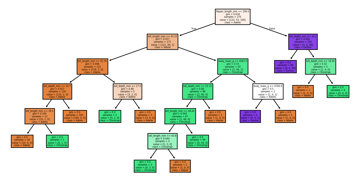

Accuracy: 0.91
Classification Report:
              precision    recall  f1-score   support

      Adelie       0.96      0.83      0.89        30
   Chinstrap       0.83      1.00      0.91        15
      Gentoo       0.92      0.96      0.94        24

    accuracy                           0.91        69
   macro avg       0.90      0.93      0.91        69
weighted avg       0.92      0.91      0.91        69

Seed: 90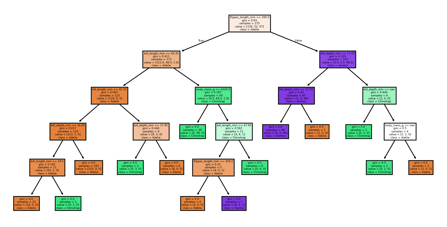

Accuracy: 0.94
Classification Report:
              precision    recall  f1-score   support

      Adelie       0.90      1.00      0.95        26
   Chinstrap       0.93      0.88      0.90        16
      Gentoo       1.00      0.93      0.96        27

    accuracy                           0.94        69
   macro avg       0.94      0.93      0.94        69
weighted avg       0.95      0.94      0.94        69

Seed: 96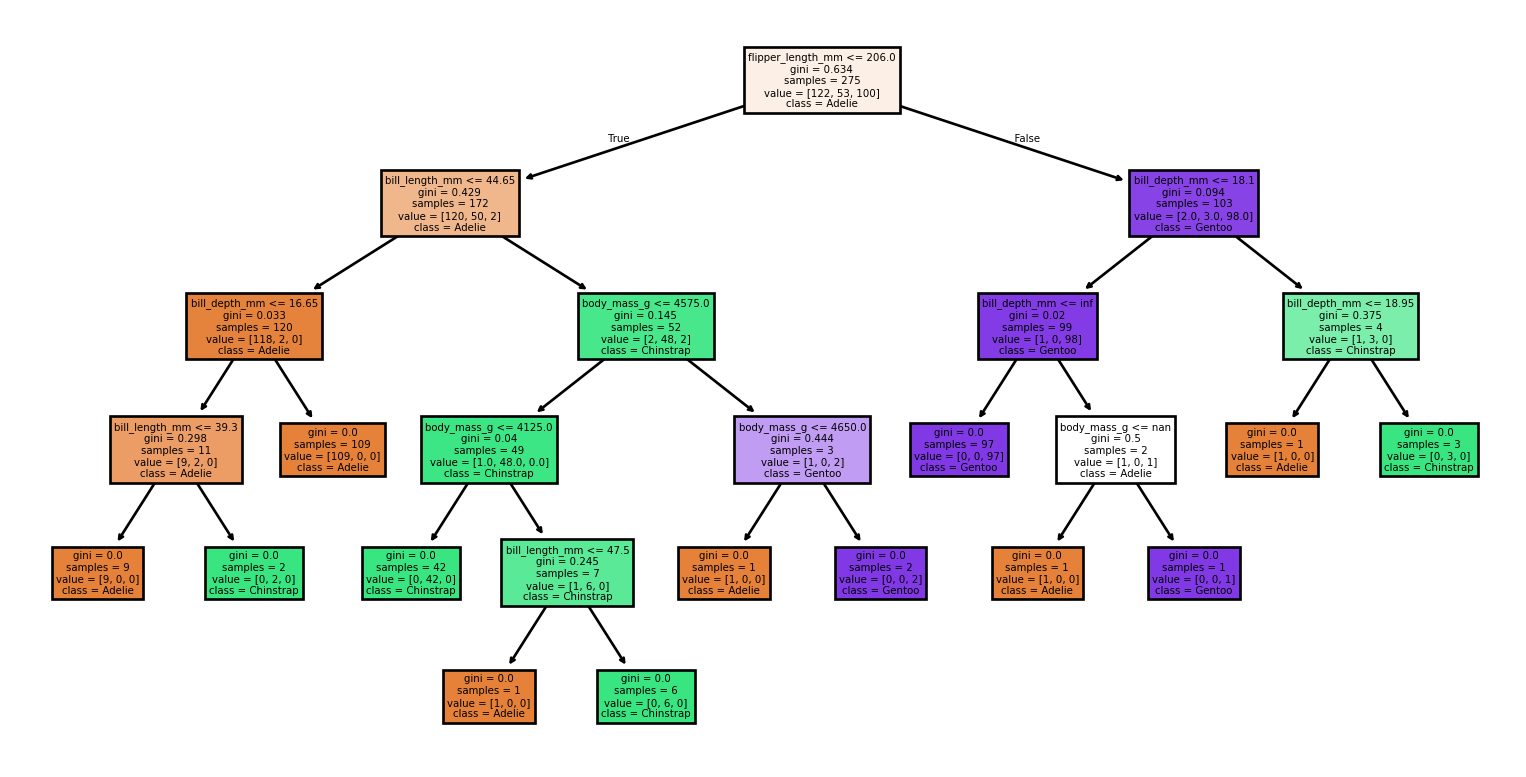

Accuracy: 0.90
Classification Report:
              precision    recall  f1-score   support

      Adelie       0.83      0.97      0.89        30
   Chinstrap       1.00      0.67      0.80        15
      Gentoo       0.96      0.96      0.96        24

    accuracy                           0.90        69
   macro avg       0.93      0.86      0.88        69
weighted avg       0.91      0.90      0.90        69

Seed: 99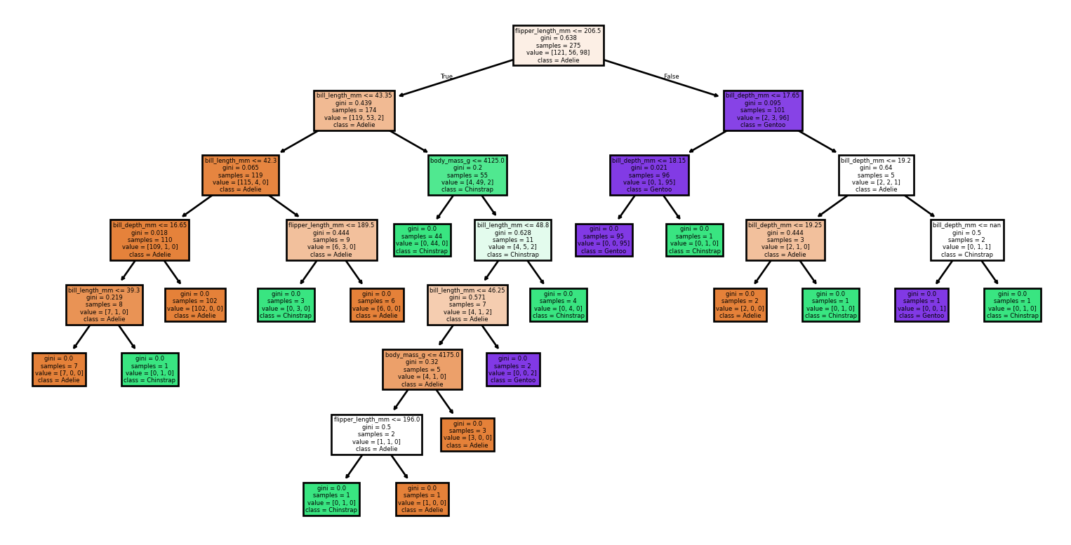

Accuracy: 1.00
Classification Report:
              precision    recall  f1-score   support

      Adelie       1.00      1.00      1.00        31
   Chinstrap       1.00      1.00      1.00        12
      Gentoo       1.00      1.00      1.00        26

    accuracy                           1.00        69
   macro avg       1.00      1.00      1.00        69
weighted avg       1.00      1.00      1.00        69

Seed: 2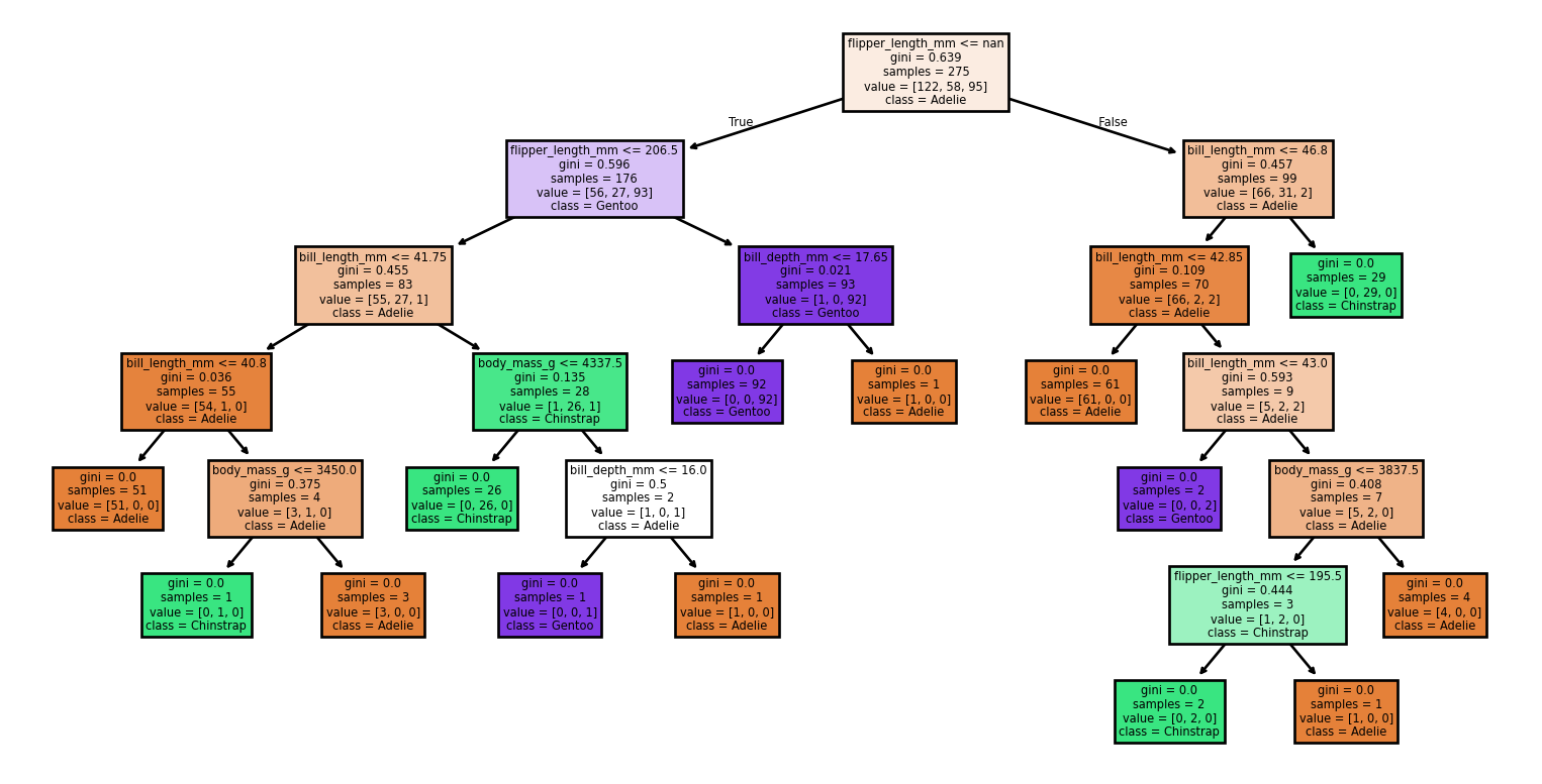

Accuracy: 0.55
Classification Report:
              precision    recall  f1-score   support

      Adelie       0.62      0.97      0.75        30
   Chinstrap       0.43      0.90      0.58        10
      Gentoo       0.00      0.00      0.00        29

    accuracy                           0.55        69
   macro avg       0.35      0.62      0.44        69
weighted avg       0.33      0.55      0.41        69

Variance

• When a classifier’s performance varies significantly across different independent test sets, it indicates that the classifier has high variance.

• High variance means that the model is very sensitive to the specific data it was trained on and may not generalize well to unseen data.

Decision Trees & Variance

• Decision Trees are known to be high variance classifiers.

• They can capture complex patterns in the training data but might also capture noise, leading to overfitting.

• Techniques like pruning, ensemble methods (such as Random Forests), and using a simpler model can help reduce variance.

Regularization

• Limiting the maximum depth of the tree is a form of regularization.
  • Likewise, the values for the other parameters, such as min_impurity_decrease, can be determined using a validation set.
• Another regularization technique for decision trees is known as pruning.
  • In a bottom-up fashion, nodes are removed if this reduces the classification error on the validation set.
• scikit-learn.org/dev/auto_examples/tree/plot_cost_complexity_pruning.html

Implementations

• ID3 (Iterative Dichotomiser 3), C4.5, C5.0 — by Ross Quinlan.
• CART (Classification And Regression Tree) — by Leo Breiman et al.
• sklearn.tree.DecisionTreeClassifier
  • https://scikit-learn.org/stable/modules/tree.html

Random Forest

Random Forest

• Ensemble methods will be discussed with greater details later.
• “Although single decision trees can be excellent classifiers, increased accuracy often can be achieved by combining the results of a collection of decision trees.” (Kingsford and Salzberg 2008)

Random Forest

• A Random Forest is a collection of decision trees.
  • Strategies to build a collection of trees:
    • Creating new data sets using a sampling with replacement procedure (bootstrap sampling);
    • Using a random subset of the features for splitting (typically the square root of the total number of features);
    • Taking advantage of the stochastic nature of the procedure to build trees.

Random Forest

• Prediction: the most common prediction (majority vote) amongst all the trees (the information can be used as an indication of the strength of the prediction).

Ensemble Learning

• Other ensemble learning techniques, such as bagging, pasting, boosting, and stacking will be discussed later.

Bagging, short for Bootstrap Aggregating, is an ensemble learning technique in machine learning aimed at reducing variance and improving model stability. It involves training multiple decision trees on different subsets of the training data, each subset created through random sampling with replacement. The predictions of these individual trees are then aggregated, typically by voting for classification or averaging for regression, to produce a final output. This approach enhances model robustness and accuracy by mitigating the effects of overfitting inherent in single decision trees.

Murphy Figure 18.4 (a)

# Baggging decision trees in 2d
# Source: https://github.com/probml/pyprobml/blob/master/notebooks/book1/18/bagging_trees.ipynb
# Based on https://github.com/ageron/handson-ml2/blob/master/06_decision_trees.ipynb

import numpy as np
import matplotlib.pyplot as plt
import os

from sklearn.metrics import accuracy_score

from sklearn.ensemble import BaggingClassifier
from sklearn.tree import DecisionTreeClassifier

from matplotlib.colors import ListedColormap

from sklearn.model_selection import train_test_split
from sklearn.datasets import make_moons

X, y = make_moons(n_samples=500, noise=0.30, random_state=42)
X_train, X_test, y_train, y_test = train_test_split(X, y, random_state=42)

def plot_decision_boundary(clf, X, y, axes=[-1.5, 2.45, -1, 1.5], alpha=0.5, contour=True):
    x1s = np.linspace(axes[0], axes[1], 100)
    x2s = np.linspace(axes[2], axes[3], 100)
    x1, x2 = np.meshgrid(x1s, x2s)
    X_new = np.c_[x1.ravel(), x2.ravel()]
    y_pred = clf.predict(X_new).reshape(x1.shape)
    custom_cmap = ListedColormap(["#fafab0", "#9898ff", "#a0faa0"])
    plt.contourf(x1, x2, y_pred, alpha=0.3, cmap=custom_cmap)
    if contour:
        custom_cmap2 = ListedColormap(["#7d7d58", "#4c4c7f", "#507d50"])
        plt.contour(x1, x2, y_pred, cmap=custom_cmap2, alpha=0.8)
    plt.plot(X[:, 0][y == 0], X[:, 1][y == 0], "yo", alpha=alpha)
    plt.plot(X[:, 0][y == 1], X[:, 1][y == 1], "bs", alpha=alpha)
    plt.axis(axes)
    plt.xlabel(r"$x_1$", fontsize=18)
    plt.ylabel(r"$x_2$", fontsize=18, rotation=0)

tree_clf = DecisionTreeClassifier(random_state=42)
tree_clf.fit(X_train, y_train)
y_pred_tree = tree_clf.predict(X_test)
dtree_acc = accuracy_score(y_test, y_pred_tree)

plt.figure()
plot_decision_boundary(tree_clf, X, y)
plt.title("Decision Tree, test accuracy={:0.2f}".format(dtree_acc))
# plt.savefig("figures/dtree_bag_size0.pdf", dpi=300)
plt.show()

Murphy (2022) PDF 2024-11-23, Figure 18.4 (a), bagging_trees.ipynb

Murphy Figure 18.4 (a)

BaggingClassifier

A Bagging classifier is an ensemble meta-estimator that fits base classifiers each on random subsets of the original dataset and then aggregate their individual predictions (either by voting or by averaging) to form a final prediction.

BaggingClassifier

BaggingClassifier

When random subsets of the dataset are drawn as random subsets of the samples, then this algorithm is known as Pasting. If samples are drawn with replacement, then the method is known as Bagging. When random subsets of the dataset are drawn as random subsets of the features, then the method is known as Random Subspaces. Finally, when base estimators are built on subsets of both samples and features, then the method is known as Random Patches.

BaggingClassifier

Murphy Figure 18.4 (c)

# bag_sizes = [10, 50, 100]
bag_sizes = [50]

for bag_size in bag_sizes:
    bag_clf = BaggingClassifier(
        DecisionTreeClassifier(random_state=42), n_estimators=bag_size, max_samples=100, bootstrap=True, random_state=42
    )
    bag_clf.fit(X_train, y_train)
    y_pred = bag_clf.predict(X_test)
    bag_acc = accuracy_score(y_test, y_pred)

    plt.figure()
    plot_decision_boundary(bag_clf, X, y)
    plt.title("Bag of {} decision trees, test accuracy={:0.2f}".format(bag_size, bag_acc))
    # plt.savefig("figures/dtree_bag_size{}.pdf".format(bag_size), dpi=300)
    plt.show()

Murphy (2022) PDF 2024-11-23, Figure 18.4 (c), bagging_trees.ipynb

Murphy Figure 18.4 (c)

Applications

SingleCellNet

• Multi-class Random Forest classifier to classify single-cell RNA-seq data across different platforms and species.

• Shown to be resilient to confounding factors, such as the cell cycle stage, which often affects clustering analysis in scRNA-seq data.

• SCN-TP outperforms other methods like SCMAP in terms of mean AUPR and classification accuracy.

1. Cross-Platform and Cross-Species Classification: SCN is a computational tool designed to classify single-cell RNA-seq data across different platforms and species, which is a significant advancement in the field of bioinformatics and machine learning for biological data.

2. Top-Pair Transformation and Random Forest: The method uses a novel approach called Top-Pair transformation, where gene expression data is transformed into a binary matrix based on pairwise comparisons of selected genes. This transformation is followed by training a multi-class Random Forest classifier, which is a robust machine learning technique.

3. Performance Metrics: The performance of SCN is evaluated using metrics like Cohen’s kappa and mean area under the precision-recall curve (mean AUPR), demonstrating its effectiveness in classification tasks.

4. Resilience to Biological Confounders: SCN-TP (Top-Pair) is shown to be resilient to confounding factors such as the cell cycle stage, which often affects clustering analysis in scRNA-seq data.

5. Comparison with Other Methods: SCN-TP outperforms other methods like SCMAP in terms of mean AUPR and classification accuracy, highlighting its superior performance in cross-platform and cross-species scenarios.

These findings illustrate the application of machine learning techniques, such as Random Forests and data transformation, to solve complex biological classification problems, making it a relevant study for a machine learning course.

(Tan and Cahan 2019)

Applications in bioinformatics

• Synthetic sick and lethal (SSL) genetic interactions between genes A and B occur when the organism exhibits poor growth (or death) when both A and B are knocked out but not when either A or B is disabled individually. (Kingsford and Salzberg 2008)

• Determine the exon-intron structure of eukaryotic genes (gene finders). (Kingsford and Salzberg 2008)

• In the study of gene expression profiling. (Kingsford and Salzberg 2008)

• Cancer classification (Barlin et al. 2013).

Resources

• XGBoost, eXtreme Gradient Boosting, documentation.
• LightGBM, includes GPU-based learning.

Nearest-Neighbor (Placeholder)

Prologue

Summary

Decision trees can perform both classification and regression, readily handling categorical and numerical attributes without relying on rigid assumptions about the data. They offer high interpretability but can suffer from instability and overfitting, issues often mitigated by pruning or ensemble methods like random forests. Overall, decision trees remain a foundational tool in machine learning, used in everything from gene expression analysis to clinical diagnostics.

Next Lecture

• Linear models

References

Barlin, Joyce N., Qin Zhou, Caryn M. St. Clair, Alexia Iasonos, Robert A. Soslow, Kaled M. Alektiar, Martee L. Hensley, Mario M. Leitao, Richard R. Barakat, and Nadeem R. Abu-Rustum. 2013. “Classification and regression tree (CART) analysis of endometrial carcinoma: Seeing the forest for the trees.” Gynecologic Oncology 130 (3): 452–56. https://doi.org/10.1016/j.ygyno.2013.06.009.

Géron, Aurélien. 2019. Hands-on Machine Learning with Scikit-Learn, Keras, and TensorFlow. 2nd ed. O’Reilly Media.

Geurts, Pierre, Alexandre Irrthum, and Louis Wehenkel. 2009. “Supervised Learning with Decision Tree-Based Methods in Computational and Systems Biology.” Molecular bioSystems 5 (12): 1593–1605. https://doi.org/10.1039/b907946g.

Hyafil, Laurent, and Ronald L. Rivest. 1976. “Constructing Optimal Binary Decision Trees Is NP-Complete.” Inf. Process. Lett. 5 (1): 15–17. https://doi.org/10.1016/0020-0190(76)90095-8.

Kingsford, C, and Steven L Salzberg. 2008. “What Are Decision Trees?” Nature Biotechnology 26 (9): 1011–13. https://doi.org/10.1038/nbt0908-1011.

Leboeuf, Jean-Samuel, Frédéric LeBlanc, and Mario Marchand. 2022. “Generalization Properties of Decision Trees on Real-Valued and Categorical Features.” https://arxiv.org/abs/2210.10781.

Murphy, Kevin P. 2022. Probabilistic Machine Learning: An Introduction. MIT Press. http://probml.github.io/book1.

Schietgat, Leander, Celine Vens, Jan Struyf, Hendrik Blockeel, Dragi Kocev, and Saso Dzeroski. 2010. “Predicting Gene Function Using Hierarchical Multi-Label Decision Tree Ensembles.” BMC Bioinformatics 11 (1): 2. https://doi.org/10.1186/1471-2105-11-2.

Stiglic, Gregor, Simon Kocbek, Igor Pernek, and Peter Kokol. 2012. “Comprehensive Decision Tree Models in Bioinformatics.” Edited by Ahmed Moustafa. PLoS ONE 7 (3): e33812. https://doi.org/10.1371/journal.pone.0033812.

Tan, Yuqi, and Patrick Cahan. 2019. “SingleCellNet: A Computational Tool to Classify Single Cell RNA-Seq Data Across Platforms and Across Species.” Cell Systems 9 (2): 207–213.e2. https://doi.org/10.1016/j.cels.2019.06.004.

Marcel Turcotte

Marcel.Turcotte@uOttawa.ca

School of Electrical Engineering and Computer Science (EECS)

University of Ottawa