Linear models, training

CSI 5180 - Machine Learning for Bioinformatics

Marcel Turcotte

Version: Feb 19, 2025 13:30

Preamble

Quote of the Day

Ten simple rules to complete successfully a computational MSc thesis project

(Saccenti and Furlan 2025)

Quote of the Day

“Eric Topol has published over 1300 peer-reviewed articles, with more than 300,000 citations, elected to the National Academy of Medicine, and is one of the top 10 most cited researchers in medicine. His principal scientific focus has been on the use of genomic and digital data, along with artificial intelligence, to individualize medicine. He is also a practicing cardiologist.”

(Topol 2025)

Training a Linear Model

In this lecture, we will cover the foundational concepts of linear regression, and gradient descent.

You will gain a deeper understanding of these essential machine learning techniques, enabling you to apply them effectively in your work.

General Objective

• Explain the process of training a linear model

Learning Objectives

• Distinguish between regression and classification tasks.
• Explain the training process for linear regression models.
• In your own words, explain the role of optimization algorithms in solving linear regression problems.
• Describe the role of partial derivatives in the gradient descent algorithm.
• Compare the batch, stochastic, and mini-batch gradient descent algorithms.

Readings

• Based on Géron (2019), \(\S\) 4.

Problem

Supervised Learning - Regression

• The training data is a collection of labelled examples.
  • \(\{(x_i,y_i)\}_{i=1}^N\)
    • Each \(x_i\) is a feature vector with \(D\) dimensions.
    • \(x_i^{(j)}\) is the value of the feature \(j\) of the example \(i\), for \(j \in 1 \ldots D\) and \(i \in 1 \ldots N\).
  • The label \(y_i\) is a real number.
• Problem: Given the data set as input, create a model that can be used to predict the value of \(y\) for an unseen \(x\).

Rationale

Linear regression is introduced to conveniently present a well-known training algorithm, gradient descent. Additionally, it serves as a foundation for introducing logistic regression–a classification algorithm—which further facilitates discussions on artificial neural networks.

• Linear Regression
  • Gradient Descent
  • Logistic Regression
    • Neural Networks

The training algorithms for machine learning models can vary significantly depending on the model (e.g., decision trees, SVMs, etc.). In order to fit our schedule, we will concentrate on this specific sequence.

The concept of linear regression can be traced back to the early work of Sir Francis Galton in the late 19th century. Galton introduced the idea of “regression” in his 1886 paper, which focused on the relationship between the heights of parents and their children. He observed that children’s heights tended to regress towards the average, which led to the term “regression.”

However, the mathematical formulation of linear regression is closely associated with the work of Karl Pearson, who in the early 20th century extended Galton’s ideas to create the method of least squares for fitting a linear model. The method itself, though, was developed earlier in 1805 by Adrien-Marie Legendre and independently by Carl Friedrich Gauss for astronomical data analysis.

See: Stanton (2001).

Linear Regression

• A linear model assumes that the value of the label, \(\hat{y_i}\), can be expressed as a linear combination of the feature values, \(x_i^{(j)}\): \[ \hat{y_i} = h(x_i) = \theta_0 + \theta_1 x_i^{(1)} + \theta_2 x_i^{(2)} + \ldots + \theta_D x_i^{(D)} \]
  
• Here, \(\theta_{j}\) is the \(j\)th parameter of the (linear) model, with \(\theta_0\) being the bias term/parameter, and \(\theta_1 \ldots \theta_D\) being the feature weights.

Example

Linear Regression Example

• Gene Expression Level Prediction:
  • Study: “Inferring epigenetic and transcriptional regulation during blood cell development”
  • Summary: This research employs a mixture of sparse linear regression models to predict gene expression levels based on transcription factor binding and histone modification signals, enhancing understanding of regulatory mechanisms in hematopoiesis.

(Rego et al. 2012) [data]

Gene Regulation

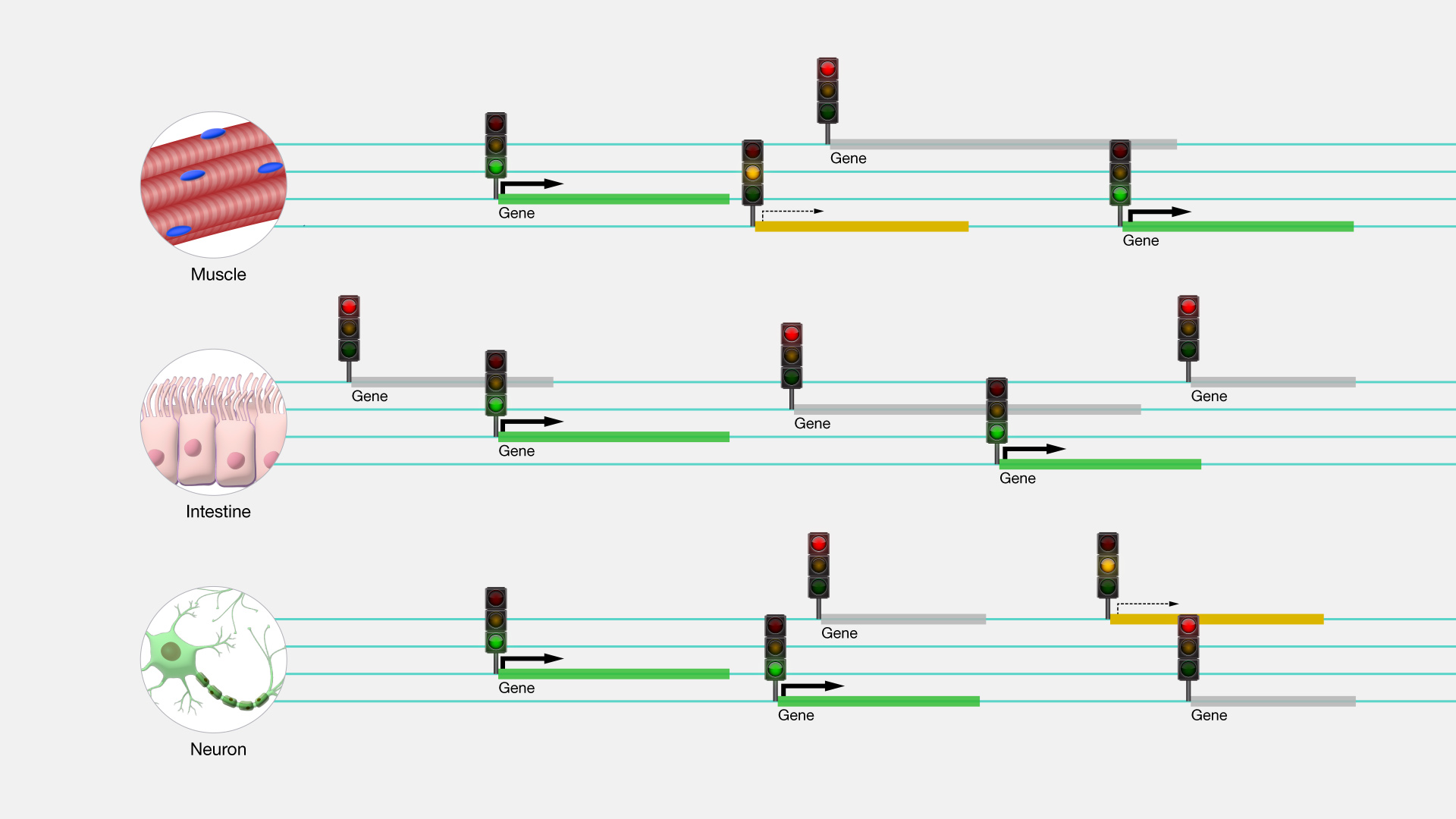
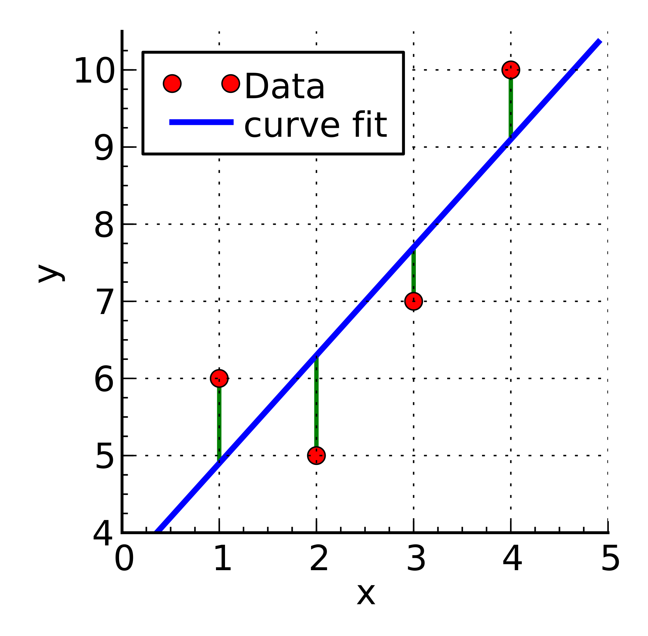
Gene regulation at the National Human Genome Research Institute

Gene regulation is the process used to control the timing, location and amount in which genes are expressed.

Epigenetics

Centers for Disease Control and Prevention 2024-04-20

Your genes play an important role in your health, but so do your behaviors and environment, such as what you eat and how physically active you are. Epigenetics is the study of how your behaviors and environment can cause changes that affect the way your genes work. Unlike genetic changes, epigenetic changes are reversible and do not change your DNA sequence, but they can change how your body reads a DNA sequence.

Gene expression refers to how often or when proteins are created from the instructions within your genes. While genetic changes can alter which protein is made, epigenetic changes affect gene expression to turn genes “on” and “off.” Since your environment and behaviors, such as diet and exercise, can result in epigenetic changes, it is easy to see the connection between your genes and your behaviors and environment.

Epigenetics

• “Epigenetics is the study of heritable changes in gene expression (active versus inactive gene) that do not involve changes to the underlying DNA sequence — a change in phenotype without a change in genotype — which in turn affects how cells read the genes.”

• “Epigenetic change is a regular and natural occurrence but can also be influenced by several factors including age, the environment/lifestyle, and disease state.”

• “Epigenetic modifications can manifest as commonly as the manner in which cells terminally differentiate to end up as skin cells, liver cells, brain cells, etc.”

• “At least three systems including methylation, histone modifications and non-coding RNA (ncRNA).”

Phenotype refers to the observable characteristics or traits of an organism, resulting from the interaction of its genotype with the environment. These traits include physical attributes, biochemical properties, and behavioral tendencies.

Genotype refers to the genetic constitution of an organism, encompassing the specific alleles and genetic information encoded in its DNA that determine inherited traits and potential phenotypic expression.

What is epigenetics?

Epigenetics

What is epigenetics?

Mixture of Sparse Linear Regressions

• \(y_i\) is the expression level of gene \(i\).

• \(x_i = \{x_{i1},\ldots,x_{iP}\}\) is a vector with \(P\) regulatory signals for gene \(i\).

• where \(i=1,\ldots,N\).

• The learned coefficients identify whether a signal functions as an activator (positive), a repressor (negative), or is irrelevant (zero).

“Schematic blood cell developmental tree (top) and a sample mixture model inferred on the MPP cell (bottom). The mixture model predicts the gene expression of genes of a particular cell type Y —depicted as a red–green bar—by the regulatory signals of the genes X —depicted as the blue–white plot, where blue values indicate a higher presence of the histone in a gene promoter. The coefficients B indicate the roles of each regulatory signal. The mixture of sparse linear regression search for groups of genes, whose expression are determined by the same regulatory network. For example, model 1 predicts genes with high expression and indicates that H3k4me3 and H3k79me2 are activators of expression and H3k27me3 and H3k27me3 are repressors of expression. The elastic net method gives similar coefficients to co-linear signals, such as the pairs H3k79me2/H3k4me3 and H3k27me3/H3k9me3. Also, irrelevant signals, such as H3ac are removed, i.e. have the coefficient set to 0. Note that distinct models indicate distinct regulatory elements. For model 2, only the HMs H3k4me3, H3k79me2 and H3kac were selected as relevant for determining the activity of low expressed genes.”

See New paradigms on hematopoietic stem cell differentiation for additional information on the differentiation roadmap of blood cells.

Data Overview

• Transcription Factor Affinity Calculation: The TRAP method is employed to quantify the affinity of transcription factor \(j\) for the promoter region of gene \(i\). This results in features denoted as \(x_{i,j}\), where \(j\) ranges from 1 to 599.
• Histone Mark Profiles: ChIP-chip data, sourced from GEO, provide histone mark profiles for H3K4me, H3K79me2, H3ac, H3K9me3, and H3K27me3. These are also represented as \(x_{i,j}\), with \(j\) spanning from 1 to 5.
• Gene Expression Data: Affymetrix mRNA expression data, obtained from GEO, are utilized to measure gene expression levels, denoted as \(y_i\), \(i \in 1,\ldots,4,089\).
• Cell Types Analyzed: The study encompasses four distinct cell types: Hematopoietic Stem Cells (HSC), Multipotent Progenitor Cells (MPP), Pre-Megakaryocyte/Erythroid Progenitors (PreMegE), and T Helper Cells (TCD4).

Design

• Employed transcription factor (TF) affinities, histone marks (HM), or a combination of TF and HM as regulatory signals denoted by \(x_{i,j}\).
• Adjusted the number of linear models in the range of 1 to 10.
• Modified \(L_1\) and \(L_2\) regularization parameters within Elastic Net regression to manage sparsity effectively.

In gene expression, a regulatory program refers to the network of interactions and mechanisms by which genes are activated or repressed in response to various internal and external signals, involving transcription factors, enhancers, silencers, and other regulatory elements that control the timing, location, and level of gene expression.

Results

• Optimal Models: Two regression models were determined to be optimal.
  • “Interestingly, the two linear models always separate the data into high and low expression genes on all blood cells.”
• Hematopoietic Stem Cells (HSC):
  • Histone Marks (HM): 4 of 5 selected.
  • Transcription Factors (TF): 67 of 599 selected.
  • Regulatory Signals: 39 of 604 selected when incorporating TF/HM data.

Summary

1. The paper introduces a methodology for predicting gene expression based on an extensive array of regulatory signals, including transcription factor binding affinities and histone modification profiles.

2. The approach autonomously determines the optimal number of regression models required for accurate predictions.

3. It also automatically selects pertinent features, enhancing model precision.

Building Blocks

Supervised Learning - Regression

• The training data is a collection of labelled examples.
  • \(\{(x_i,y_i)\}_{i=1}^N\)
    • Each \(x_i\) is a feature vector with \(D\) dimensions.
    • \(x_i^{(j)}\) is the value of the feature \(j\) of the example \(i\),\ for \(j \in 1 \ldots D\) and \(i \in 1 \ldots N\).
  • The label \(y_i\) is a real number.
• Problem: Given the data set as input, create a model that can be used to predict the value of \(y\) for an unseen \(x\).

Characteristics

A typical learning algorithm comprises the following components:

1. A model, often consisting of a set of weights whose values will be “learnt”.
2. An objective function.
   • In the case of regression, this is often a loss function, a function that quantifies misclassification. The Root Mean Square Error is a common loss function for regression problems. \(\sqrt{\frac{1}{N}\sum_1^N [h(x_i) - y_i]^2}\)
3. Optimization algorithm

Linear Regression

• A linear model assumes that the value of the label, \(\hat{y_i}\), can be expressed as a linear combination of the feature values, \(x_i^{(j)}\): \[ \hat{y_i} = h(x_i) = \theta_0 + \theta_1 x_i^{(1)} + \theta_2 x_i^{(2)} + \ldots + \theta_D x_i^{(D)} \]
  
• Here, \(\theta_{j}\) is the \(j\)th parameter of the (linear) model, with \(\theta_0\) being the bias term/parameter, and \(\theta_1 \ldots \theta_D\) being the feature weights.

Linear Regression (continued)

Problem: find values for all the model parameters so that the model “best fits” the training data.

• The Root Mean Square Error is a common performance measure for regression problems.

\[ \sqrt{\frac{1}{N}\sum_1^N [h(x_i) - y_i]^2} \]

Linear Regression (continued)

Attribution: Krishnavedala, CC BY-SA 3.0, via Wikimedia Commons

Optimization

Until some termination criteria is met¹:

• Evaluate the loss function, comparing \(h(x_i)\) to \(y_i\).
• Make small changes to the weights, in a way that reduces the value of the loss function.

1. E.g. the value of the loss function no longer decreases or the maximum number of iterations.

Remarks

• It is crucial to separate the optimization algorithm from the problem it addresses.
• For linear regression, although exact analytical solution exists, but it presents certain limitations.
• Gradient descent serves as a general algorithm applicable not only to linear regression but also to logistic regression, deep learning, t-SNE (t-distributed Stochastic Neighbor Embedding), among various other problems.
• There exists a diverse range of optimization algorithms that do not rely on gradient-based methods.

Derivative

from sympy import *
from matplotlib import style
style.use('seaborn-v0_8-whitegrid')

t = symbols('t')

f = t**2 + 4*t + 7

plot(f, size=(5, 5))

• We will start with a single-variable function.
• Think of this as our loss function, which we aim to minimize; to reduce the average discrepancy between expected and predicted values.
• Here, I am using \(t\) to avoid any confusion with the attributes of our training examples.

I’ve used SymPy, a library for symbolic mathematics.

Derivative

import sympy as sp
import numpy as np
import matplotlib.pyplot as plt

# Define the variable and function
t = sp.symbols('t')
f = t**2 + 4*t + 7

# Compute the derivative
f_prime = sp.diff(f, t)

# Lambdify the functions for numerical plotting
f_func = sp.lambdify(t, f, "numpy")
f_prime_func = sp.lambdify(t, f_prime, "numpy")

# Generate t values for plotting
t_vals = np.linspace(-5, 2, 400)

# Get y values for the function and its derivative
f_vals = f_func(t_vals)
f_prime_vals = f_prime_func(t_vals)

# Plot the function and its derivative
plt.plot(t_vals, f_vals, label=r'$f(t) = t^2 + 4t + 7$', color='blue')
plt.plot(t_vals, f_prime_vals, label=r"$f'(t) = 2t + 4$", color='red')

# Add labels and legend
plt.axhline(0, color='black',linewidth=1)
plt.axvline(0, color='black',linewidth=1)
plt.title('Function and Derivative')
plt.xlabel('t')
plt.ylabel(r'$f(t)$')
plt.legend()

# Show the plot
plt.grid(True)
plt.show()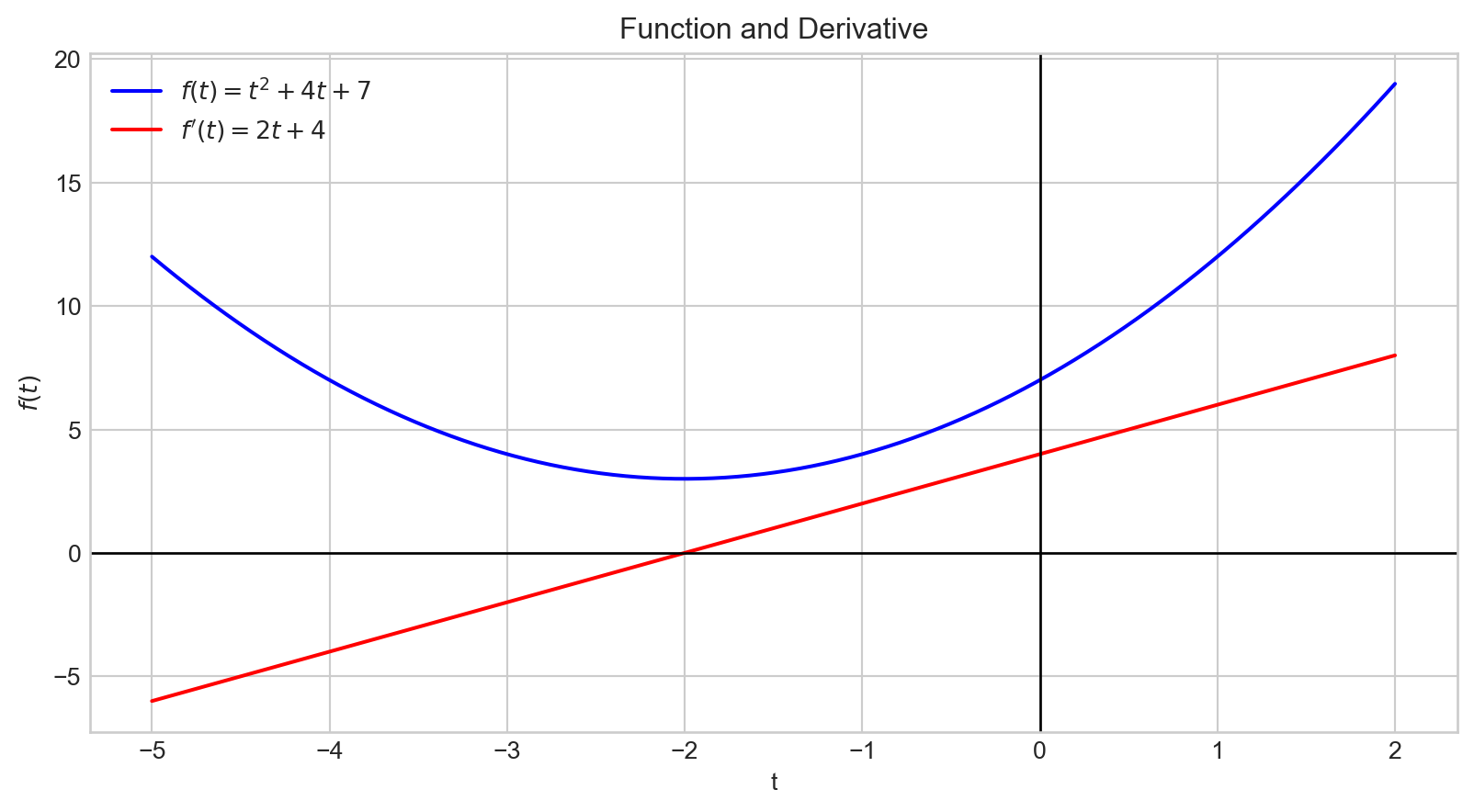

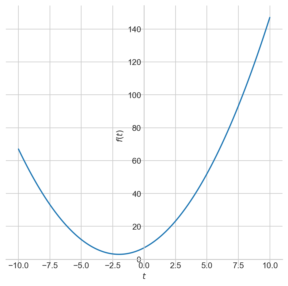
• The graph of the derivative, \(f^{'}(t)\), is depicted in red.

• The derivative indicates how changes in the input affect the output, \(f(t)\).

• The magnitude of the derivative at \(t = -2\) is \(0\).

• This point corresponds to the minimum of our function.

In traditional calculus, you may be accustomed to interpreting the derivative as the slope of the tangent line at a specific point \(t\). Here, I will introduce this concept from an alternative perspective.

Near \(t = -2\), variations in \(t\) have minimal impact on the output, \(f(t)\).

Derivative

import sympy as sp
import numpy as np
import matplotlib.pyplot as plt

# Define the variable and function
t = sp.symbols('t')
f = t**2 + 4*t + 7

# Compute the derivative
f_prime = sp.diff(f, t)

# Lambdify the functions for numerical plotting
f_func = sp.lambdify(t, f, "numpy")
f_prime_func = sp.lambdify(t, f_prime, "numpy")

# Generate t values for plotting
t_vals = np.linspace(-5, 2, 400)

# Get y values for the function and its derivative
f_vals = f_func(t_vals)
f_prime_vals = f_prime_func(t_vals)

# Plot the function and its derivative
plt.plot(t_vals, f_vals, label=r'$f(t) = t^2 + 4t + 7$', color='blue')
plt.plot(t_vals, f_prime_vals, label=r"$f'(t) = 2t + 4$", color='red')

# Add labels and legend
plt.axhline(0, color='black',linewidth=1)
plt.axvline(0, color='black',linewidth=1)
plt.title('Function and Derivative')
plt.xlabel('t')
plt.ylabel('y')
plt.legend()

# Show the plot
plt.grid(True)
plt.show()

• When evaluated at a specific point, the derivative indicates the slope of the tangent line to the graph of the function at that point.
• At \(t= -2\), the slope of the tangent line is 0.

Derivative

import sympy as sp
import numpy as np
import matplotlib.pyplot as plt

# Define the variable and function
t = sp.symbols('t')
f = t**2 + 4*t + 7

# Compute the derivative
f_prime = sp.diff(f, t)

# Lambdify the functions for numerical plotting
f_func = sp.lambdify(t, f, "numpy")
f_prime_func = sp.lambdify(t, f_prime, "numpy")

# Generate t values for plotting
t_vals = np.linspace(-5, 2, 400)

# Get y values for the function and its derivative
f_vals = f_func(t_vals)
f_prime_vals = f_prime_func(t_vals)

# Plot the function and its derivative
plt.plot(t_vals, f_vals, label=r'$f(t) = t^2 + 4t + 7$', color='blue')
plt.plot(t_vals, f_prime_vals, label=r"$f'(t) = 2t + 4$", color='red')

# Fill the area below the derivative where it's negative
plt.fill_between(t_vals, f_prime_vals, where=(f_prime_vals > 0), color='red', alpha=0.3)

# Add labels and legend
plt.axhline(0, color='black',linewidth=1)
plt.axvline(0, color='black',linewidth=1)
plt.title('Function and Derivative')
plt.xlabel('t')
plt.ylabel('y')
plt.legend()

# Show the plot
plt.grid(True)
plt.show()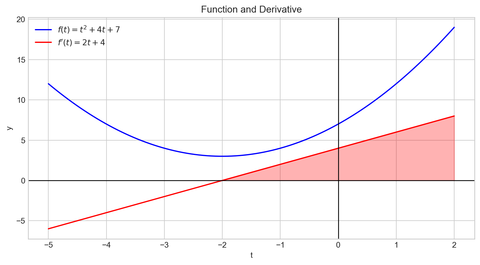

• A positive derivative indicates that increasing the input variable will increase the output value.

• Additionally, the magnitude of the derivative quantifies how rapidly the output changes.

Derivative

import sympy as sp
import numpy as np
import matplotlib.pyplot as plt

# Define the variable and function
t = sp.symbols('t')
f = t**2 + 4*t + 7

# Compute the derivative
f_prime = sp.diff(f, t)

# Lambdify the functions for numerical plotting
f_func = sp.lambdify(t, f, "numpy")
f_prime_func = sp.lambdify(t, f_prime, "numpy")

# Generate t values for plotting
t_vals = np.linspace(-5, 2, 400)

# Get y values for the function and its derivative
f_vals = f_func(t_vals)
f_prime_vals = f_prime_func(t_vals)

# Plot the function and its derivative
plt.plot(t_vals, f_vals, label=r'$f(t) = t^2 + 4t + 7$', color='blue')
plt.plot(t_vals, f_prime_vals, label=r"$f'(t) = 2t + 4$", color='red')

# Fill the area below the derivative where it's negative
plt.fill_between(t_vals, f_prime_vals, where=(f_prime_vals < 0), color='red', alpha=0.3)

# Add labels and legend
plt.axhline(0, color='black',linewidth=1)
plt.axvline(0, color='black',linewidth=1)
plt.title('Function and Derivative')
plt.xlabel('t')
plt.ylabel('y')
plt.legend()

# Show the plot
plt.grid(True)
plt.show()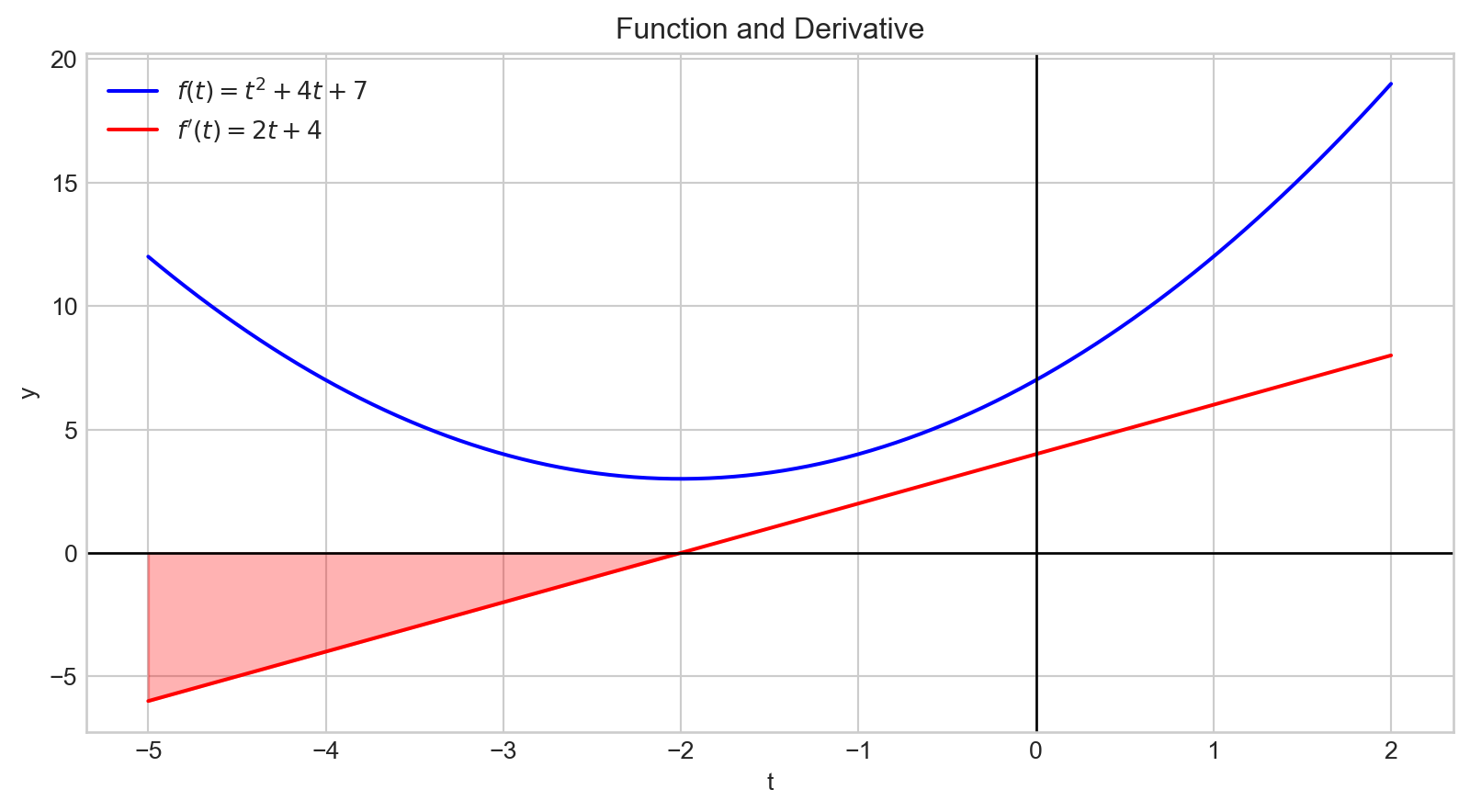

• A negative derivative indicates that increasing the input variable will decrease the output value.

• Additionally, the magnitude of the derivative quantifies how rapidly the output changes.

Recall

• A linear model assumes that the value of the label, \(\hat{y_i}\), can be expressed as a linear combination of the feature values, \(x_i^{(j)}\): \[ \hat{y_i} = h(x_i) = \theta_0 + \theta_1 x_i^{(1)} + \theta_2 x_i^{(2)} + \ldots + \theta_D x_i^{(D)} \]
  
• Here, \(\theta_{j}\) is the \(j\)th parameter of the (linear) model, with \(\theta_0\) being the bias term/parameter, and \(\theta_1 \ldots \theta_D\) being the feature weights.

Recall

• The Root Mean Square Error (RMSE) is a common loss function for regression problems. \[ \sqrt{\frac{1}{N}\sum_1^N [h(x_i) - y_i]^2} \]
• In practice, minimizing the Mean Squared Error (MSE) is easier and gives the same result. \[ \frac{1}{N}\sum_1^N [h(x_i) - y_i]^2 \]

Gradient Descent - Intuition

Gradient Descent - Step-by-Step

Gradient Descent - Single Value

• Our model: \[ h(x_i) = \theta_0 + \theta_1 x_i^{(1)} \]
• Our loss function: \[ J(\theta_0, \theta_1) = \frac{1}{N}\sum_1^N [h(x_i) - y_i]^2 \]
• Problem: find the values of \(\theta_0\) and \(\theta_1\) that minimize \(J\).

Observe that our loss function computes the sum of residuals across the entire training dataset.

Gradient Descent - Single Value

• Initialization: \(\theta_0\) and \(\theta_1\) - either with random values or zeros.
• Loop:
  • repeat until convergence: \[ \theta_j := \theta_j - \alpha \frac {\partial}{\partial \theta_j}J(\theta_0, \theta_1) , \text{for } j=0 \text{ and } j=1 \]
• \(\alpha\) is called the learning rate - this is the size of each step.
• \(\frac {\partial}{\partial \theta_j}J(\theta_0, \theta_1)\) is the partial derivative with respect to \(\theta_j\).

A partial derivative represents the rate of change of a multivariable function with respect to one of its variables, while keeping the other variables constant.

For the algorithm to be mathematically sound, all the \(\theta_j\) must be updated simultaneously.

Gradient Descent - Single Value

import sympy as sp
import numpy as np
import matplotlib.pyplot as plt

# Define the variable and function
t = sp.symbols('t')
f = t**2 + 4*t + 7

# Compute the derivative
f_prime = sp.diff(f, t)

# Lambdify the functions for numerical plotting
f_func = sp.lambdify(t, f, "numpy")
f_prime_func = sp.lambdify(t, f_prime, "numpy")

# Generate t values for plotting
t_vals = np.linspace(-5, 2, 400)

# Get y values for the function and its derivative
f_vals = f_func(t_vals)
f_prime_vals = f_prime_func(t_vals)

# Plot the function and its derivative
plt.plot(t_vals, f_vals, label=r'$J$', color='blue')
plt.plot(t_vals, f_prime_vals, label=r"$\frac {\partial}{\partial \theta_j}J(\theta)$", color='red')

# Add labels and legend
plt.axhline(0, color='black',linewidth=1)
plt.axvline(0, color='black',linewidth=1)
plt.title('Function and Derivative')
plt.xlabel(r'$\theta_j$')
plt.ylabel(r'$J$')
plt.legend()

# Show the plot
plt.grid(True)
plt.show()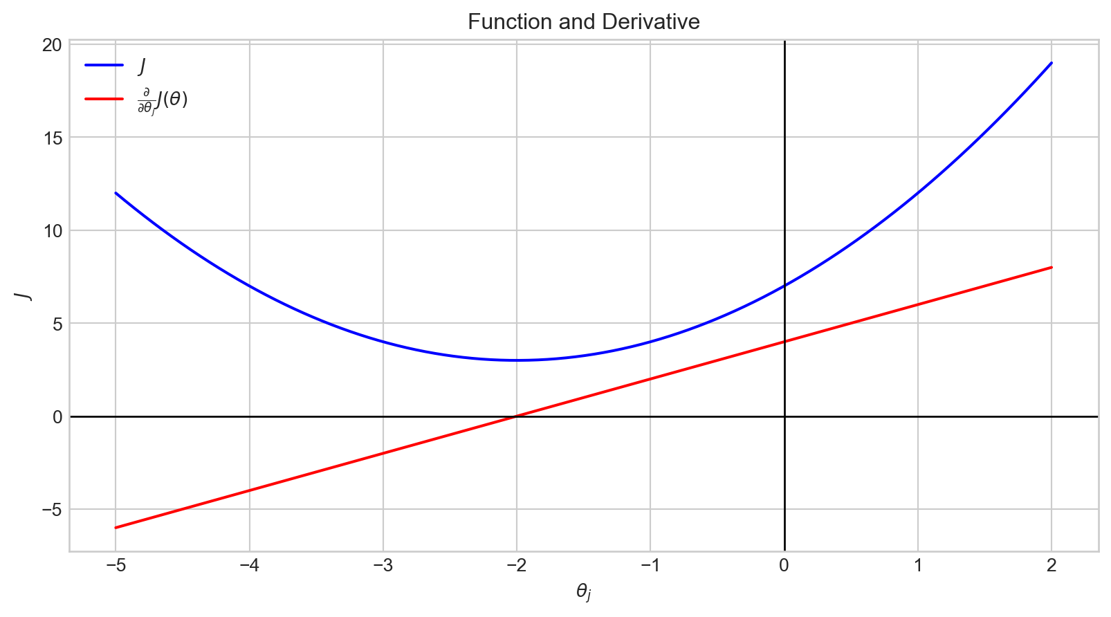

• When the value of \(\theta_j\) is in the range \([- \inf, -2)\), \(\frac {\partial}{\partial \theta_j}J(\theta)\) has a negative value.

• Therefore, \(- \alpha \frac {\partial}{\partial \theta_j}J(\theta)\) is positive.

• Accordingly, the value of \(\theta_j\) is increased.

Updating rule: \(\theta_j := \theta_j - \alpha \frac {\partial}{\partial \theta_j}J(\theta_0, \theta_1) , \text{for } j=0 \text{ and } j=1\).

Gradient Descent - Single Value

import sympy as sp
import numpy as np
import matplotlib.pyplot as plt

# Define the variable and function
t = sp.symbols('t')
f = t**2 + 4*t + 7

# Compute the derivative
f_prime = sp.diff(f, t)

# Lambdify the functions for numerical plotting
f_func = sp.lambdify(t, f, "numpy")
f_prime_func = sp.lambdify(t, f_prime, "numpy")

# Generate t values for plotting
t_vals = np.linspace(-5, 2, 400)

# Get y values for the function and its derivative
f_vals = f_func(t_vals)
f_prime_vals = f_prime_func(t_vals)

# Plot the function and its derivative
plt.plot(t_vals, f_vals, label=r'$J$', color='blue')
plt.plot(t_vals, f_prime_vals, label=r"$\frac {\partial}{\partial \theta_j}J(\theta)$", color='red')

# Add labels and legend
plt.axhline(0, color='black',linewidth=1)
plt.axvline(0, color='black',linewidth=1)
plt.title('Function and Derivative')
plt.xlabel(r'$\theta_j$')
plt.ylabel(r'$J$')
plt.legend()

# Show the plot
plt.grid(True)
plt.show()

• When the value of \(\theta_j\) is in the range \((-2, \infty]\), \(\frac {\partial}{\partial \theta_j}J(\theta)\) has a positive value.

• Therefore, \(- \alpha \frac {\partial}{\partial \theta_j}J(\theta)\) is negative.

• Accordingly, the value of \(\theta_j\) is decreased.

Updating rule: \(\theta_j := \theta_j - \alpha \frac {\partial}{\partial \theta_j}J(\theta_0, \theta_1) , \text{for } j=0 \text{ and } j=1\).

Partial Derivatives

Given

\[ J(\theta_0, \theta_1) = \frac{1}{N}\sum_1^N [h(x_i) - y_i]^2 = \frac{1}{N}\sum_1^N [\theta_0 + \theta_1 x_i - y_i]^2 \]

We have

\[ \frac {\partial}{\partial \theta_0}J(\theta_0, \theta_1) = \frac{2}{N} \sum\limits_{i=1}^{N} (\theta_0 - \theta_1 x_i - y_{i}) \]

and

\[ \frac {\partial}{\partial \theta_1}J(\theta_0, \theta_1) = \frac{2}{N} \sum\limits_{i=1}^{N} x_{i} \left(\theta_0 + \theta_1 x_i - y_{i}\right) \]

Partial Derivate (SymPy)

from IPython.display import Math, display
from sympy import *

# Define the symbols

theta_0, theta_1, x_i, y_i = symbols('theta_0 theta_1 x_i y_i')

# Define the hypothesis function:

h = theta_0 + theta_1 * x_i

print("Hypothesis function:")

display(Math('h(x) = ' + latex(h)))

Hypothesis function:

\(\displaystyle h(x) = \theta_{0} + \theta_{1} x_{i}\)

Partial Derivate (SymPy)

N = Symbol('N', integer=True)

# Define the loss function (mean squared error)

J = (1/N) * Sum((h - y_i)**2, (x_i, 1, N))

print("Loss function:")

display(Math('J = ' + latex(J)))

Loss function:

\(\displaystyle J = \frac{\sum_{x_{i}=1}^{N} \left(\theta_{0} + \theta_{1} x_{i} - y_{i}\right)^{2}}{N}\)

Partial Derivate (SymPy)

# Calculate the partial derivative with respect to theta_0

partial_derivative_theta_0 = diff(J, theta_0)

print("Partial derivative with respect to theta_0:")

display(Math(latex(partial_derivative_theta_0)))

Partial derivative with respect to theta_0:

\(\displaystyle \frac{\sum_{x_{i}=1}^{N} \left(2 \theta_{0} + 2 \theta_{1} x_{i} - 2 y_{i}\right)}{N}\)

Partial Derivate (SymPy)

# Calculate the partial derivative with respect to theta_1

partial_derivative_theta_1 = diff(J, theta_1)

print("\nPartial derivative with respect to theta_1:")

display(Math(latex(partial_derivative_theta_1)))

Partial derivative with respect to theta_1:

\(\displaystyle \frac{\sum_{x_{i}=1}^{N} 2 x_{i} \left(\theta_{0} + \theta_{1} x_{i} - y_{i}\right)}{N}\)

Multivariate Linear Regression

\[ h (x_i) = \theta_0 + \theta_1 x_i^{(1)} + \theta_2 x_i^{(2)} + \theta_3 x_i^{(3)} + \cdots + \theta_D x_i^{(D)} \]

\[ \begin{align*} x_i^{(j)} &= \text{value of the feature } j \text{ in the } i \text{th example} \\ D &= \text{the number of features} \end{align*} \]

Gradient Descent - Multivariate

The new loss function is

\[ J(\theta_0, \theta_1,\ldots,\theta_D) = \dfrac {1}{N} \displaystyle \sum _{i=1}^N \left (h(x_{i}) - y_i \right)^2 \]

Its partial derivative:

\[ \frac {\partial}{\partial \theta_j}J(\theta) = \frac{2}{N} \sum\limits_{i=1}^N x_i^{(j)} \left( \theta x_i - y_i \right) \]

where \(\theta\), \(x_i\) and \(y_i\) are vectors, and \(\theta x_i\) is a vector operation!

Gradient Vector

The vector containing the partial derivative of \(J\) (with respect to \(\theta_j\), for \(j \in \{0, 1\ldots D\}\)) is called the gradient vector.

\[ \nabla_\theta J(\theta) = \begin{pmatrix} \frac {\partial}{\partial \theta_0}J(\theta) \\ \frac {\partial}{\partial \theta_1}J(\theta) \\ \vdots \\ \frac {\partial}{\partial \theta_D}J(\theta)\\ \end{pmatrix} \]

• This vector gives the direction of the steepest ascent.
• It gives its name to the gradient descent algorithm:

\[ \theta' = \theta - \alpha \nabla_\theta J(\theta) \]

Gradient Descent - Multivariate

The gradient descent algorithm becomes:

Repeat until convergence:

\[ \begin{aligned} \{ & \\ \theta_j := & \theta_j - \alpha \frac {\partial}{\partial \theta_j}J(\theta_0, \theta_1, \ldots, \theta_D) \\ &\text{for } j \in [0, \ldots, D] \textbf{ (update simultaneously)} \\ \} & \end{aligned} \]

Gradient Descent - Multivariate

Repeat until convergence:

\[ \begin{aligned} \; \{ & \\ \; & \theta_0 := \theta_0 - \alpha \frac{2}{N} \sum\limits_{i=1}^{N} x^{0}_i(h(x_i) - y_i) \\ \; & \theta_1 := \theta_1 - \alpha \frac{2}{N} \sum\limits_{i=1}^{N} x^{1}_i(h(x_i) - y_i) \\ \; & \theta_2 := \theta_2 - \alpha \frac{2}{N} \sum\limits_{i=1}^{N} x^{2}_i(h(x_i) - y_i) \\ & \cdots \\ \} & \end{aligned} \]

Assumptions

What were our assumptions?

• The (objective/loss) function is differentiable.

Local vs. Global

• A function is convex if for any pair of points on the graph of the function, the line connecting these two points lies above or on the graph.

  • A convex function has a single minimum.
    • The loss function for the linear regression (MSE) is convex.

• For functions that are not convex, the gradient descent algorithm converges to a local minimum.

• The loss function generally used with linear or logistic regressions, and Support Vector Machines (SVM) are convex, but not the ones for artificial neural networks.

A function would be convex downward or concave if those lines were below or on the graph of the function.

Local vs. Global

Attribution: commons.wikimedia.org/wiki/File:Extrema_example.svg

Convergence

# 1. Define the symbolic variable and the function
x = sp.Symbol('x', real=True)
f_expr = 2*x**3 + 4*x**2 - 5*x + 1

# 2. Compute the derivative of f
f_prime_expr = sp.diff(f_expr, x)

# 3. Convert symbolic expressions to Python functions
f = sp.lambdify(x, f_expr, 'numpy')
f_prime = sp.lambdify(x, f_prime_expr, 'numpy')

# 4. Generate a range of x-values
x_vals = np.linspace(-4, 2, 1000)

# 5. Compute f and f' over this range
y_vals = f(x_vals)
y_prime_vals = f_prime(x_vals)

# 6. Prepare LaTeX strings for legend
f_label = rf'$f(x) = {sp.latex(f_expr)}$'
f_prime_label = rf'$f^\prime(x) = {sp.latex(f_prime_expr)}$'

# 7. Plot f and f', with equations in the legend
plt.figure(figsize=(8, 4))
plt.plot(x_vals, y_vals, label=f_label)
plt.plot(x_vals, y_prime_vals, label=f_prime_label)

# 8. Shade the region between x-axis and f'(x) for the entire domain
plt.fill_between(x_vals, y_prime_vals, 0, color='gray', alpha=0.2, interpolate=True,
                 label='Region between 0 and f\'(x)')

# 9. Add reference line, labels, legend, etc.
plt.axhline(0, color='black', linewidth=0.5)
plt.title(rf'Function and its Derivative with Shading for $f^\prime(x)$')
plt.xlabel('x')
plt.ylabel('y')
plt.legend()
plt.grid(True)
plt.show()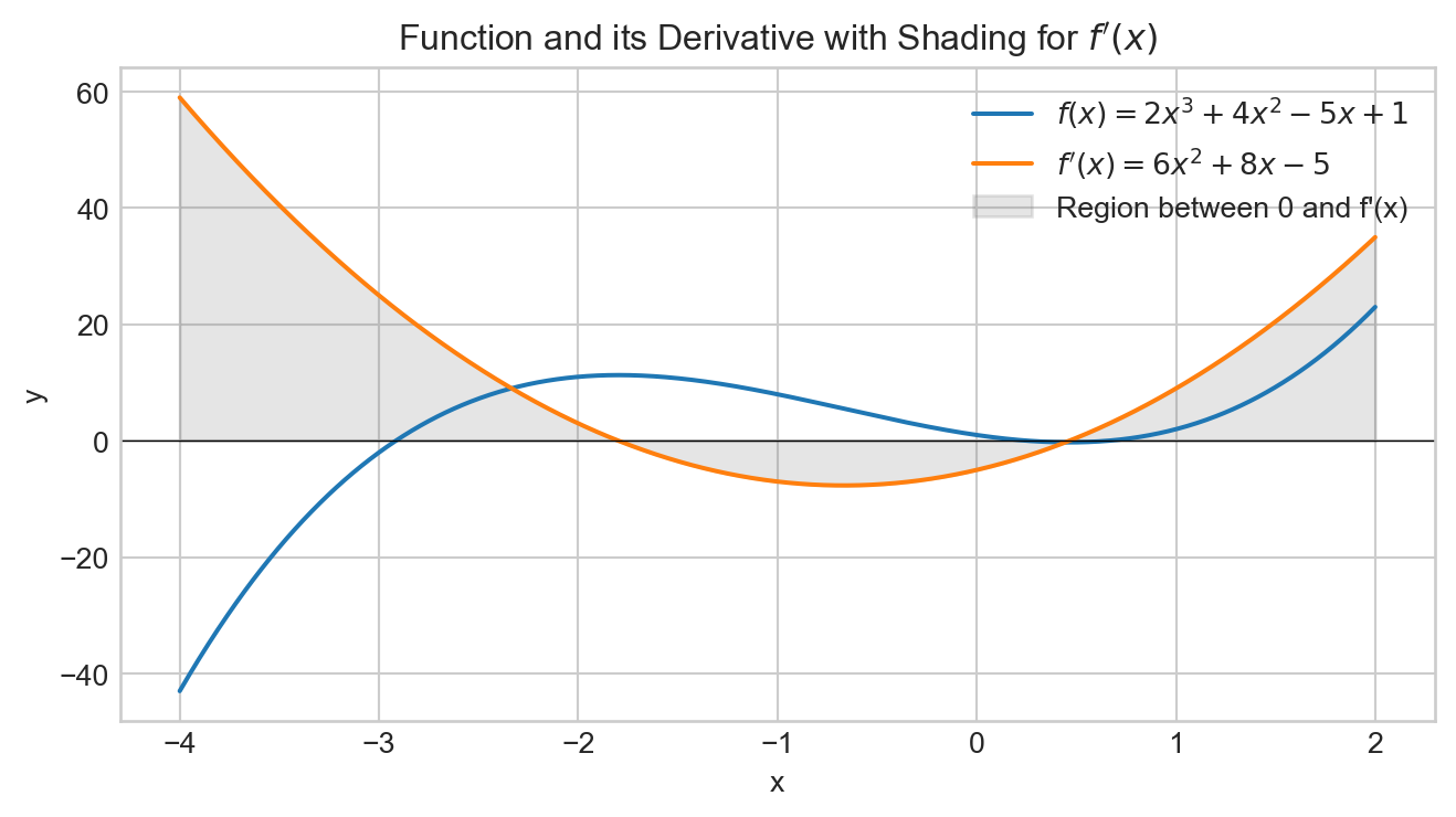

• The first objective of this example is to illustrate that gradient descent is applicable to functions of arbitrary complexity, provided that the gradient can be computed or approximated at each iteration.

• Furthermore, the function must possesses at least one local minimum within the interval of interest.

For functions lacking a global minimum, gradient descent can continue descending indefinitely, preventing convergence.

Learning Rate

• Small steps, low values for \(\alpha\), will make the algorithm converge slowly.
• Large steps might cause the algorithm to diverge.
• Notice how the algorithm slows down naturally when approaching a minimum.

Learning Rate

import numpy as np
import matplotlib.pyplot as plt

def f(x):
    return x**2

def grad_f(x):
    return 2*x

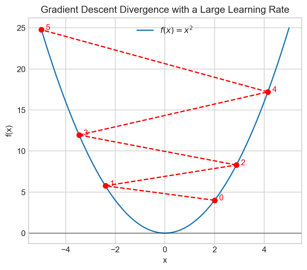
# Initial guess, learning rate, and number of gradient-descent steps
x_current = 2.0
learning_rate = 1.1  # Too large => divergence
num_iterations = 5   # We'll do five updates

# Store each x value in a list (trajectory) for plotting
trajectory = [x_current]

# Perform gradient descent
for _ in range(num_iterations):
    g = grad_f(x_current)
    x_current = x_current - learning_rate * g
    trajectory.append(x_current)

# Prepare data for plotting
x_vals = np.linspace(-5, 5, 1000)
y_vals = f(x_vals)

# Plot the function f(x)
plt.figure(figsize=(6, 5))
plt.plot(x_vals, y_vals, label=r"$f(x) = x^2$")
plt.axhline(0, color='black', linewidth=0.5)

# Plot the trajectory, labeling each iteration
for i, x_t in enumerate(trajectory):
    y_t = f(x_t)
    # Plot the point
    plt.plot(x_t, y_t, 'ro')
    # Label the iteration number
    plt.text(x_t, y_t, f"  {i}", color='red')
    # Connect consecutive points
    if i > 0:
        x_prev = trajectory[i - 1]
        y_prev = f(x_prev)
        plt.plot([x_prev, x_t], [y_prev, y_t], 'r--')

# Final touches
plt.title("Gradient Descent Divergence with a Large Learning Rate")
plt.xlabel("x")
plt.ylabel("f(x)")
plt.legend()
plt.grid(True)
plt.show()

Batch Gradient Descent

• To be more precise, this algorithm is known as batch gradient descent since for each iteration, it processes the “whole batch” of training examples.

• Literature suggests that the algorithm might take more time to converge if the features are on different scales.

Batch Gradient descent - Drawback

• The batch gradient descent algorithm becomes very slow as the number of training examples increases.

• This is because all the training data is seen at each iteration. The algorithm is generally run for a fixed number of iterations, say 1000.

Stochastic Gradient Descent

The stochastic gradient descent algorithm randomly selects one training instance to calculate its gradient.

epochs = 10
for epoch in range(epochs):
   for i in range(N):
         selection = np.random.randint(N)
         # Calculate the gradient using selection
         # Update the weights

• This allows it to work with large training sets.
• Its trajectory is not as regular as the batch algorithm.
  • Because of its bumpy trajectory, it is often better at finding the global minima, when compared to batch.
  • Its bumpy trajectory makes it bounce around the local minima.

To mitigate the issue of oscillating around local minima, it is advisable to progressively reduce the learning rate as the number of epochs increases. This technique, known as a learning schedule, helps achieve more stable convergence.

It important that the examples are either selected randomly or shuffled before running the algorithm to make sure that the algorithm converges towards the global minima.

Stochastic Gradient Descent

Attribution: Krishnavedala, CC BY-SA 3.0, via Wikimedia Commons

Mini-Batch Gradient Descent

• At each step, rather than selecting one training example as SGD does, mini-batch gradient descent randomly selects a small number of training examples to compute the gradients.
• Its trajectory is more regular compared to SGD.
  • As the size of the mini-batches increases, the algorithm becomes increasingly similar to batch gradient descent, which uses all the examples at each step.
• It can take advantage of the hardware acceleration of matrix operations, particularly with GPUs.

Summary

• Batch gradient descent is inherently slow and impractical for large datasets requiring out-of-core support, though it is capable of handling a substantial number of features.

• Stochastic gradient descent is fast and well-suited for processing a large volume of examples efficiently.

• Mini-batch gradient descent combines the benefits of both batch and stochastic methods; it is fast, capable of managing large datasets, and leverages hardware acceleration, particularly with GPUs.

The typical size of a mini-batch when applying stochastic gradient descent (SGD) can vary depending on the specific application and dataset, but common sizes often range between 32 and 512 samples. Here are some common mini-batch sizes used in practice:

1. Small Mini-Batches: Sizes such as 16, 32, or 64 are often used when working with smaller datasets or when memory constraints are a concern.
2. Medium Mini-Batches: Sizes like 128, 256, or 512 are commonly used and can provide a good balance between computational efficiency and convergence speed.
3. Large Mini-Batches: Sizes like 1024, 2048, or larger might be used in large-scale machine learning tasks, especially when sufficient computational resources are available.

The choice of mini-batch size can influence several factors such as:

• Training Speed: Larger mini-batches can make better use of parallel processing capabilities, potentially speeding up training.
• Convergence: Smaller mini-batches can introduce more noise in the gradient estimation, which can sometimes help escape local minima and improve generalization.
• Memory Usage: Larger mini-batches require more memory, which might be a limiting factor, especially on GPUs with limited VRAM.

Ultimately, the optimal mini-batch size is task-specific and often determined empirically through experimentation.

All three are implemented by SGDRegressor in Scikit-Learn.

Fundamentals by Herman Kamper

Optimization and Deep Nets

We will briefly revisit the subject when discussing deep artificial neural networks, for which specialized optimization algorithms exist.

• Momentum Optimization
• Nesterov Accelerated Gradient
• AdaGrad
• RMSProp
• Adam and Nadam

Final Word

• Optimization is a vast subject. Other algorithms exist and are used in other contexts.
  • Including:
    • Particle swarm optimization (PSO), genetic algorithms (GAs), and artificial bee colony (ABC) algorithms.

Linear Regression - Summary

• A linear model assumes that the value of the label, \(\hat{y_i}\), can be expressed as a linear combination of the feature values, \(x_i^{(j)}\): \(\hat{y_i} = h(x_i) = \theta_0 + \theta_1 x_i^{(1)} + \theta_2 x_i^{(2)} + \ldots + \theta_D x_i^{(D)}\)
• The Mean Squared Error (MSE) is: \(\frac{1}{N}\sum_1^N [h(x_i) - y_i]^2\)
• Batch, stochastic, or mini-batch gradient descent can be used to find “optimal” values for the weights, \(\theta_j\) for \(j \in 0, 1, \ldots, D\).
• The result is a regressor, a function that can be used to predict the \(y\) value (the label) for some unseen example \(x\).

Prologue

References

Géron, Aurélien. 2019. Hands-on Machine Learning with Scikit-Learn, Keras, and TensorFlow. 2nd ed. O’Reilly Media.

Rego, Thais G. do, Helge G. Roider, Francisco A. T. de Carvalho, and Ivan G. Costa. 2012. “Inferring epigenetic and transcriptional regulation during blood cell development with a mixture of sparse linear models.” Bioinformatics 28 (18): 2297–2303. https://doi.org/10.1093/bioinformatics/bts362.

Saccenti, Edoardo, and Cristina Furlan. 2025. “Ten simple rules to complete successfully a computational MSc thesis project.” PLOS Computational Biology 21 (1): e1012756. https://doi.org/10.1371/journal.pcbi.1012756.

Stanton, Jeffrey M. 2001. “Galton, Pearson, and the Peas: A Brief History of Linear Regression for Statistics Instructors.” Journal of Statistics Education 9 (3). https://doi.org/10.1080/10691898.2001.11910537.

Topol, Eric J. 2025. “Learning the Language of Life with AI.” Science 387 (6733): eadv4414. https://doi.org/10.1126/science.adv4414.

Next lecture

• Part 2 of linear models, logistic regression

Appendix

Normal Equation

The closed-form analytical solution to the linear regression problem is known as the normal equation.

1. Computational Complexity: Calculating the inverse of \(X^T X\) has a time complexity of \(O(n^3)\) (web.cs.ucla.edu).

2. Numerical Stability: If \(X^T X\) is nearly singular or ill-conditioned, inversion can lead to significant numerical errors (cs.cornell.edu).

3. Memory Requirements: The matrix \(X^T X\) has dimensions \(n \times n\), which can be prohibitive in terms of memory usage when \(n\) is large (web.cs.ucla.edu).

It is important to note that the normal equation is applicable to linear regression models only.

LinearRegression

import numpy as np

X = 6 * np.random.rand(100, 1) - 4
y = X ** 2 - 4 * X + 5 + np.random.randn(100, 1)

from sklearn.linear_model import LinearRegression

lin_reg = LinearRegression()
lin_reg.fit(X, y)

X_new = np.array([[-4], [2]])
y_pred = lin_reg.predict(X_new)

import matplotlib as mpl
import matplotlib.pyplot as plt

plt.plot(X, y, "b.")
plt.plot(X_new, y_pred, "r-")
plt.xlabel("$x$", fontsize=18)
plt.ylabel("$y$", rotation=0, fontsize=18)
plt.axis([-4, 2, -1, 35])
# save_fig("regression_linear-01")
plt.show()

from sklearn.linear_model import LinearRegression

lin_reg = LinearRegression()
lin_reg.fit(X, y)

Herein, we examine a straightforward model involving a single variable.

LinearRegression

Source Code

import numpy as np

X = 6 * np.random.rand(100, 1) - 4
y = X ** 2 - 4 * X + 5 + np.random.randn(100, 1)

from sklearn.linear_model import LinearRegression

lin_reg = LinearRegression()
lin_reg.fit(X, y)

X_new = np.array([[-4], [2]])
y_pred = lin_reg.predict(X_new)

The data have been generated from a quadratic model, \(x^2 - 4x + 5\), with Gaussian noise added to make the synthetic data more realistic.

This example illustrates that, in practice, we often have limited knowledge about the underlying model that generated the data.

Despite this uncertainty, we make assumptions—in this case, assuming linearity—when building our models.

Later, we will refer to this as bias (distinct from the bias parameter in our regression model). Both bias and variance influence the performance of our models.

This slide contains an anomaly. Can you identify it?

GPT 4o interactions (2024-09-14)

User: Explain the code on the previous slide line by line.

AI: Certainly! Here is a line-by-line explanation of the provided code:

import numpy as np

• Explanation: This line imports the NumPy library, which is a fundamental package for numerical computations in Python. It is commonly used for working with arrays and matrices, as well as for performing a variety of mathematical operations.

X = 6 * np.random.rand(100, 1) - 4

• Explanation: This line generates a NumPy array X containing 100 rows and 1 column of random numbers. The np.random.rand(100, 1) function generates uniformly distributed random numbers between 0 and 1. Multiplying by 6 scales these numbers to the range [0, 6), and subtracting 4 shifts the range to [-4, 2).

y = X ** 2 - 4 * X + 5 + np.random.randn(100, 1)

• Explanation: This line generates the target variable y based on a quadratic equation with some added noise. Specifically:
  • X ** 2 computes the square of each element in X.
  • - 4 * X subtracts four times each element in X.
  • + 5 adds a constant term of 5.
  • + np.random.randn(100, 1) adds Gaussian noise with a mean of 0 and standard deviation of 1 to each element, making the data more realistic by introducing some randomness.

from sklearn.linear_model import LinearRegression

• Explanation: This line imports the LinearRegression class from the sklearn.linear_model module, which is part of the Scikit-Learn library. Scikit-Learn is widely used for machine learning in Python.

lin_reg = LinearRegression()

• Explanation: This line creates an instance of the LinearRegression class and assigns it to the variable lin_reg. This object will be used to fit the linear regression model to the data.

lin_reg.fit(X, y)

• Explanation: This line fits the linear regression model to the data by finding the best-fitting line through the points (X, y). The fit method trains the model using the provided features X and target variable y.

X_new = np.array([[-4], [2]])

• Explanation: This line creates a new NumPy array X_new with two values: -4 and 2. These values represent new data points for which we want to predict the target variable using the trained model.

y_pred = lin_reg.predict(X_new)

• Explanation: This line uses the trained linear regression model to predict the target variable y_pred for the new data points in X_new. The predict method returns the predicted values based on the fitted model.

In summary, this script generates synthetic data, fits a linear regression model to it, and then uses the model to make predictions on new data points.

Marcel Turcotte

Marcel.Turcotte@uOttawa.ca

School of Electrical Engineering and Computer Science (EECS)

University of Ottawa