Linear models, Logistic Regression (Part 2)

CSI 5180 - Machine Learning for Bioinformatics

Marcel Turcotte

Version: Feb 19, 2025 11:45

Preamble

Quote of the Day

Julie Delon, Université Paris Descartes

In high dimensional spaces, nobody can hear you scream.

From this lecture on the “curse of dimensionality”, visited on 2025-02-06. See page 11.

Summary

This lecture explores linear models to classification using logistic regression. It explains converting linear feature combinations into probabilities with the sigmoid function and minimizing cross-entropy loss via gradient descent. It also covers decision boundary geometry, extends to multiclass classification with one-vs-all, and includes practical implementations like synthetic data and handwritten digit recognition, with visualizations.

Learning Outcomes

• Explain logistic regression and its probabilistic interpretation using the sigmoid function.
  
• Derive and implement the cross-entropy loss (negative log-likelihood) and its gradient for parameter estimation.
  
• Apply gradient descent to optimize logistic regression models for binary and multiclass tasks.
  
• Extend binary logistic regression to multiclass classification via one-vs-all strategies.
  
• Visualize decision boundaries and interpret weight vectors in high-dimensional feature spaces.

Loss Function

Model Overview

• Our model is expressed in a vectorized form as:

  \[ h_\theta(x_i) = \sigma(\theta x_i) = \frac{1}{1+e^{- \theta x_i}} \]

• Prediction:

  • Assign \(y_i = 0\), if \(h_\theta(x_i) < 0.5\); \(y_i = 1\), if \(h_\theta(x_i) \geq 0.5\)

• The parameter vector \(\theta\) is optimized using gradient descent.

• Which loss function should be used and why?

In logistic regression, the output is regarded as a probability, with particular emphasis on the interpretation process.

Remarks

• In constructing machine learning models with libraries like scikit-learn or keras, one has to select a loss function or accept the default one.

• Initially, the terminology can be confusing, as identical functions may be referenced by various names.

• Our aim is to elucidate these complexities.

• It is actually not that complicated!

Parameter Estimation

• Logistic regression is statistical model.

• Its output is \(\hat{y} = P(y = 1 | x, \theta)\).

• \(P(y = 0 | x, \theta) = 1 - \hat{y}\).

• Assumes that \(y\) values come from a Bernoulli distribution.

• \(\theta\) is commonly found by Maximum Likelihood Estimation.

The expressions \(\hat{y}\), \(h_\theta(x_i)\), and \(\sigma(\theta x_i)\) represent the same concept, albeit at varying levels of abstraction and specificity.

Parameter Estimation

Maximum Likelihood Estimation (MLE) is a statistical method used to estimate the parameters of a probabilistic model.

It identifies the parameter values that maximize the likelihood function, which measures how well the model explains the observed data.

Likelihood Function

Assuming the \(y\) values are independent and identically distributed (i.i.d.), the likelihood function is expressed as the product of individual probabilities.

In other words, given our data, \(\{(x_i, y_i)\}_{i=1}^N\), the likelihood function is given by this equation. \[ \mathcal{L}(\theta) = \prod_{i=1}^{N} P(y_i \mid x_i, \theta) \]

Maximum Likelihood

\[ \hat{\theta} = \underset{\theta \in \Theta}{\arg \max} \mathcal{L}(\theta) = \underset{\theta \in \Theta}{\arg \max} \prod_{i=1}^{N} P(y_i \mid x_i, \theta) \]

• Observations:

  1. Maximizing a function is equivalent to minimizing its negative.
  2. The logarithm of a product equals the sum of its logarithms.

Negative Log-Likelihood

Maximum likelihood \[ \hat{\theta} = \underset{\theta \in \Theta}{\arg \max} \mathcal{L}(\theta) = \underset{\theta \in \Theta}{\arg \max} \prod_{i=1}^{N} P(y_i \mid x_i, \theta) \]

becomes negative log-likelihood

\[ - \log \mathcal{L(\theta)} = - \log \prod_{i=1}^{N} P(y_i \mid x_i, \theta) = - \sum_{i=1}^{N} \log P(y_i \mid x_i, \theta) \]

Mathematical Reformulation

For binary outcomes, the probability \(P(y \mid x, \theta)\) is:

\[ P(y \mid x, \theta) = \begin{cases} \sigma(\theta x), & \text{if}\ y = 1 \\ 1 - \sigma(\theta x), & \text{if}\ y = 0 \end{cases} \]

This can be compactly expressed as:

\[ P(y \mid x, \theta) = \sigma(\theta x)^y (1 - \sigma(\theta x))^{1-y} \]

This “mathematical hack” validates the rationale for the label encoding.

Loss Function

We are now ready to write our loss function.

\[ J(\theta) = - \log \mathcal{L(\theta)} = - \sum_{i=1}^{N} \log P(y_i \mid x_i, \theta) \] where \(P(y \mid x, \theta) = \sigma(\theta x)^y (1 - \sigma(\theta x))^{1-y}\).

Consequently, \[ J(\theta) = - \sum_{i=1}^{N} \log [ \sigma(\theta x_i)^{y_i} (1 - \sigma(\theta x_i))^{1-y_i} ] \]

Loss Function (continued)

Simplifying the equation. \[ J(\theta) = - \sum_{i=1}^{N} \log [ \sigma(\theta x_i)^{y_i} (1 - \sigma(\theta x_i))^{1-y_i} ] \] by distributing the \(\log\) into the square parenthesis. \[ J(\theta) = - \sum_{i=1}^{N} [ \log \sigma(\theta x_i)^{y_i} + \log (1 - \sigma(\theta x_i))^{1-y_i} ] \]

Loss Function (continued)

Simplifying the equation further. \[ J(\theta) = - \sum_{i=1}^{N} [ \log \sigma(\theta x_i)^{y_i} + \log (1 - \sigma(\theta x_i))^{1-y_i} ] \] by moving the exponents in front of the \(\log\)s.

\[ J(\theta) = - \sum_{i=1}^{N} [ y_i \log \sigma(\theta x_i) + (1-y_i) \log (1 - \sigma(\theta x_i)) ] \]

The rationale for these additional simplifications will be elucidated shortly.

One More Thing

• Decision tree algorithms often employ entropy, a measure from information theory, to evaluate the quality of splits or partitions in decision rules.
• Entropy quantifies the uncertainty or impurity associated with the potential outcomes of a random variable.

Entropy

Entropy in information theory quantifies the uncertainty or unpredictability of a random variable’s possible outcomes. It measures the average amount of information produced by a stochastic source of data and is typically expressed in bits for binary systems. The entropy \(H\) of a discrete random variable \(X\) with possible outcomes \(\{x_1, x_2, \ldots, x_n\}\) and probability mass function \(P(X)\) is given by:

\[ H(X) = -\sum_{i=1}^n P(x_i) \log_2 P(x_i) \]

Cross-Entropy

Cross-entropy quantifies the difference between two probability distributions, typically the true distribution and a predicted distribution.

\[ H(p, q) = -\sum_{i} p(x_i) \log q(x_i) \] where \(p(x_i)\) is the true probability distribution, and \(q(x_i)\) is the predicted probability distribution.

Cross-Entropy

• Consider \(y\) as the true probability distribution and \(\hat{y}\) as the predicted probability distribution.
• Cross-entropy quantifies the discrepancy between these two distributions.

Cross-Entropy

Consider the negative log-likelihood loss function:

\[ J(\theta) = - \sum_{i=1}^{N} \left[ y_i \log \sigma(\theta x_i) + (1-y_i) \log (1 - \sigma(\theta x_i)) \right] \]

By substituting \(\sigma(\theta x_i)\) with \(\hat{y_i}\), the function becomes:

\[ J(\theta) = - \sum_{i=1}^{N} \left[ y_i \log \hat{y_i} + (1-y_i) \log (1 - \hat{y_i}) \right] \]

This expression illustrates that the negative log-likelihood is optimized by minimizing the cross-entropy.

Interpret the final equation as applying to all examples from 1 to \(N\) and all classes from 1 to \(k\). Here, \(k=0\) because we are addressing a binary classification problem.

Cross-entropy, log loss, and negative log-likelihood refer to the same concept.

For Each Example

import matplotlib.pyplot as plt
import numpy as np

np.random.seed(42)

# Generate an array of p values from just above 0 to 1
p_values = np.linspace(0.001, 1, 1000)

# Compute the natural logarithm of each p value
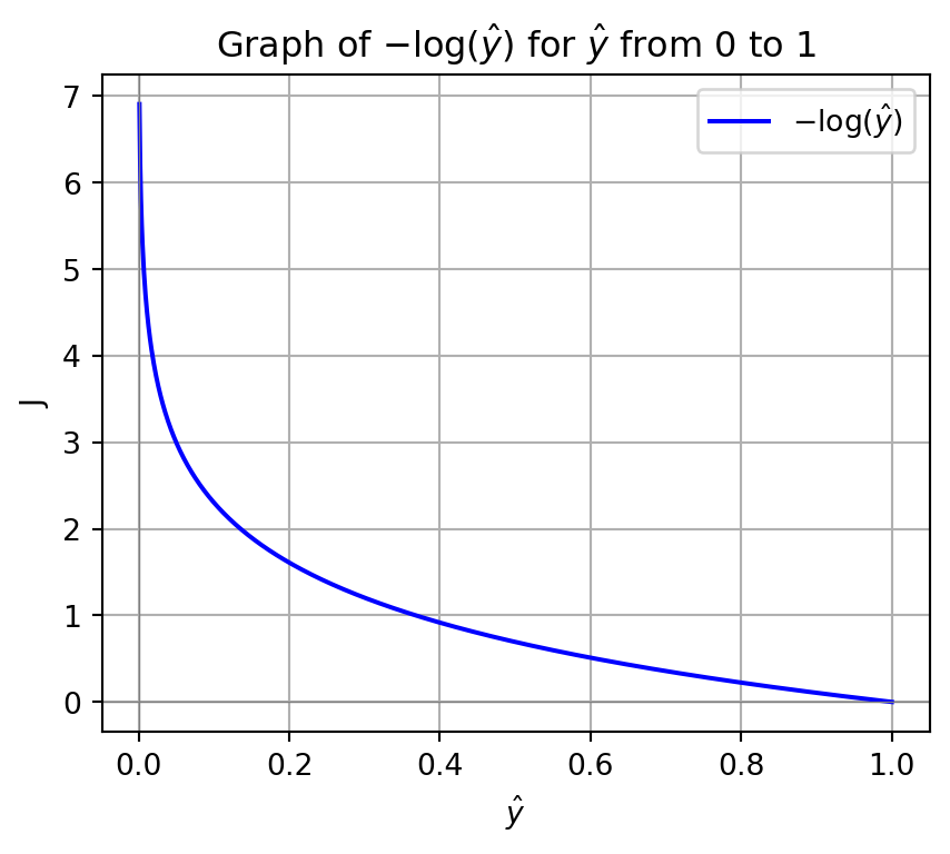
ln_p_values = - np.log(p_values)

# Plot the graph
plt.figure(figsize=(5, 4))
plt.plot(p_values, ln_p_values, label=r'$-\log(\hat{y})$', color='b')

# Add labels and title
plt.xlabel(r'$\hat{y}$')
plt.ylabel(r'J')
plt.title(r'Graph of $-\log(\hat{y})$ for $\hat{y}$ from 0 to 1')
plt.grid(True)
plt.axhline(0, color='gray', lw=0.5)  # Add horizontal line at y=0
plt.axvline(0, color='gray', lw=0.5)  # Add vertical line at x=0

# Display the plot
plt.legend()
plt.show()

For each example:

• Only one of the two terms in the summation is not zero.
• \(1 - \hat{y_i}\) is \(P(y = 0 \mid x, \theta)\).
• As \(\hat{y_i}\) tends to 1.0, \(- \log(\hat{y})\) tends to zero.
• As \(\hat{y_i}\) tends to 0.0, indicating an incorrect prediction, \(- \log(\hat{y})\) tends to \(\infty\).
• This substantial penalty allows cross-entropy loss to converge more quickly than mean squared error.

\[ J(\theta) = - \sum_{i=1}^{N} \left[ y_i \log \hat{y_i} + (1-y_i) \log (1 - \hat{y_i}) \right] \]

Remarks

• Cross-entropy loss is particularly well-suited for probabilistic classification tasks due to its alignment with maximum likelihood estimation.

• In logistic regression, cross-entropy loss preserves convexity, contrasting with the non-convex nature of mean squared error (MSE)¹.

We will revisite cross-entropy loss when studying deep learning, especially in conjunction with the softmax function.

1. In linear regression, mean squared error loss is convex.

Remarks

• For classification problems, cross-entropy loss often achieves faster convergence compared to MSE, enhancing model efficiency.

• Within deep learning architectures, MSE can exacerbate the vanishing gradient problem, an issue we will address in a subsequent discussion.

Why not MSE as a Loss Function?

What is the Difference?

Implementation

Implementation: Generating Data

# Generate synthetic data for a binary classification problem

m = 100  # number of examples
d = 2    # number of featues

X = np.random.randn(m, d)

# Define labels using a linear decision boundary with some noise:

noise = 0.5 * np.random.randn(m)

y = (X[:, 0] + X[:, 1] + noise > 0).astype(int)

Implementation: Vizualization

# Visualize the decision boundary along with the data points
plt.figure(figsize=(8, 6))
plt.scatter(X[y == 0][:, 0], X[y == 0][:, 1], color='red', label='Class 0')
plt.scatter(X[y == 1][:, 0], X[y == 1][:, 1], color='blue', label='Class 1')

plt.xlabel("Feature 1")
plt.ylabel("Feature 2")
plt.title("Data")
plt.legend()
plt.show()

Implementation: Cost Function

# Sigmoid function
def sigmoid(z):
    return 1 / (1 + np.exp(-z))

# Cost function: binary cross-entropy
def cost_function(theta, X, y):
    m = len(y)
    h = sigmoid(X.dot(theta))
    epsilon = 1e-5  # avoid log(0)
    cost = -(1/m) * np.sum(y * np.log(h + epsilon) + (1 - y) * np.log(1 - h + epsilon))
    return cost

# Gradient of the cost function
def gradient(theta, X, y):
    m = len(y)
    h = sigmoid(X.dot(theta))
    grad = (1/m) * X.T.dot(h - y)
    return grad

Implementation: Logistic Regression

# Logistic regression training using gradient descent
def logistic_regression(X, y, learning_rate=0.1, iterations=1000):
    m, n = X.shape
    theta = np.zeros(n)
    cost_history = []
    
    for i in range(iterations):
        theta -= learning_rate * gradient(theta, X, y)
        cost_history.append(cost_function(theta, X, y))
        
    return theta, cost_history

Training

# Add intercept term (bias)
X_with_intercept = np.hstack([np.ones((m, 1)), X])

# Train the logistic regression model
theta, cost_history = logistic_regression(X_with_intercept, y, learning_rate=0.1, iterations=1000)

print("Optimized theta:", theta)

Optimized theta: [-0.28840995  2.80390104  2.45238752]

Cost Function Convergence

plt.figure(figsize=(8, 6))
plt.plot(cost_history, label="Cost")
plt.xlabel("Iteration")
plt.ylabel("Cost")
plt.title("Cost Function Convergence")
plt.legend()
plt.show()

Decision Boundary and Data Points

plt.figure(figsize=(8, 6))
plt.scatter(X[y == 0][:, 0], X[y == 0][:, 1], color='red', label='Class 0')
plt.scatter(X[y == 1][:, 0], X[y == 1][:, 1], color='blue', label='Class 1')

# Decision boundary: theta0 + theta1*x1 + theta2*x2 = 0
x_vals = np.array([min(X[:, 0]) - 1, max(X[:, 0]) + 1])
y_vals = -(theta[0] + theta[1] * x_vals) / theta[2]
plt.plot(x_vals, y_vals, label='Decision Boundary', color='green')
plt.xlabel("Feature 1")
plt.ylabel("Feature 2")
plt.title("Logistic Regression Decision Boundary")
plt.legend()
plt.show()

Implementation (continued)

# Predict function: returns class labels and probabilities for new data
def predict(theta, X, threshold=0.5):
    probs = sigmoid(X.dot(theta))
    return (probs >= threshold).astype(int), probs

Predictions

# New examples must include the intercept term.

# Negative example (likely class 0): Choose a point far in the negative quadrant.
example_neg = np.array([1, -3, -3])

# Positive example (likely class 1): Choose a point far in the positive quadrant.
example_pos = np.array([1, 3, 3])

# Near decision boundary: Choose x1 = 0 and compute x2 from the decision boundary equation.
x1_near = 0
x2_near = -(theta[0] + theta[1] * x1_near) / theta[2]
example_near = np.array([1, x1_near, x2_near])

Predictions (continued)

# Combine the examples into one array for prediction.
new_examples = np.vstack([example_neg, example_pos, example_near])

labels, probabilities = predict(theta, new_examples)

print("\nPredictions on new examples:")

print("Negative example {} -> Prediction: {} (Probability: {:.4f})".format(example_neg[1:], labels[0], probabilities[0]))

print("Positive example {} -> Prediction: {} (Probability: {:.4f})".format(example_pos[1:], labels[1], probabilities[1]))

print("Near-boundary example {} -> Prediction: {} (Probability: {:.4f})".format(example_near[1:], labels[2], probabilities[2]))

Predictions on new examples:
Negative example [-3 -3] -> Prediction: 0 (Probability: 0.0000)
Positive example [3 3] -> Prediction: 1 (Probability: 1.0000)
Near-boundary example [0.         0.11760374] -> Prediction: 1 (Probability: 0.5000)

Visualizing the Weight Vector

In the previous lecture, we established that logistic regression determines a weight vector that is orthogonal to the decision boundary.

Conversely, the decision boundary itself is orthogonal to the weight vector, which is derived through gradient descent optimization.

Visualizing the Weight Vector

# Plot decision boundary and data points
plt.figure(figsize=(8, 6))
plt.scatter(X[y == 0][:, 0], X[y == 0][:, 1], color='red', label='Class 0')
plt.scatter(X[y == 1][:, 0], X[y == 1][:, 1], color='blue', label='Class 1')

# Decision boundary: theta0 + theta1*x1 + theta2*x2 = 0
x_vals = np.array([min(X[:, 0]) - 1, max(X[:, 0]) + 1])
y_vals = -(theta[0] + theta[1] * x_vals) / theta[2]
plt.plot(x_vals, y_vals, label='Decision Boundary', color='green')

# --- Draw the normal vector ---
# The normal vector is (theta[1], theta[2]).
# Choose a reference point on the decision boundary. Here, we use x1 = 0:
x_ref = 0
y_ref = -theta[0] / theta[2]  # when x1=0, theta0 + theta2*x2=0  =>  x2=-theta0/theta2

# Create the normal vector from (theta[1], theta[2]).
normal = np.array([theta[1], theta[2]])

# Normalize and scale for display
normal_norm = np.linalg.norm(normal)
if normal_norm != 0:
    normal_unit = normal / normal_norm
else:
    normal_unit = normal
scale = 2  # adjust scale as needed
normal_display = normal_unit * scale

# Draw an arrow starting at the reference point
plt.arrow(x_ref, y_ref, normal_display[0], normal_display[1],
          head_width=0.1, head_length=0.2, fc='black', ec='black')
plt.text(x_ref + normal_display[0]*1.1, y_ref + normal_display[1]*1.1, 
         r'$(\theta_1, \theta_2)$', color='black', fontsize=12)

plt.xlabel("Feature 1")
plt.ylabel("Feature 2")
plt.title("Logistic Regression Decision Boundary and Normal Vector")
plt.legend()
plt.gca().set_aspect('equal', adjustable='box')
plt.ylim(-3, 3)
plt.show()

Near the Decision Boundary

# --- Visualization Setup ---
# Create a grid over the feature space
x1_range = np.linspace(X[:, 0].min()-1, X[:, 0].max()+1, 100)
x2_range = np.linspace(X[:, 1].min()-1, X[:, 1].max()+1, 100)
xx1, xx2 = np.meshgrid(x1_range, x2_range)

# Construct the grid input (with intercept) for predictions
grid = np.c_[np.ones(xx1.ravel().shape), xx1.ravel(), xx2.ravel()]
# Compute predicted probabilities over the grid
probs = sigmoid(grid.dot(theta)).reshape(xx1.shape)
# --- Approach 2: 2D Contour (Heatmap) Plot ---
plt.figure(figsize=(8, 6))
contour = plt.contourf(xx1, xx2, probs, cmap='spring', levels=50)
plt.colorbar(contour)
plt.xlabel('Feature x1')
plt.ylabel('Feature x2')
plt.title('Contour Plot (Heatmap) of Predicted Probabilities')
# Overlay training data
plt.scatter(X[y == 0][:, 0], X[y == 0][:, 1], color='red', edgecolor='k', label='Class 0')
plt.scatter(X[y == 1][:, 0], X[y == 1][:, 1], color='blue', edgecolor='k', label='Class 1')
plt.legend()
plt.show()

Near the Decision Boundary

# --- Approach 1: 3D Surface Plot ---
fig = plt.figure(figsize=(10, 8))
ax = fig.add_subplot(111, projection='3d')
surface = ax.plot_surface(xx1, xx2, probs, cmap='spring', alpha=0.8)
ax.set_xlabel('Feature x1')
ax.set_ylabel('Feature x2')
ax.set_zlabel('Probability')
ax.set_title('3D Surface Plot of Logistic Regression Model')
fig.colorbar(surface, shrink=0.5, aspect=5)
plt.show()

“StatQuest breaks down complicated Statistics and Machine Learning methods into small, bite-sized pieces that are easy to understand. StatQuest doesn’t dumb down the material, instead, it builds you up so that you are smarter and have a better understanding of Statistics and Machine Learning.” It is often a good place to start to get the intuition to understand statistical and machine learning concepts.

Attribution: StatQuest: Logistic Regression by Josh Starmer.

Digits example

1989 Yann LeCun

Handwritten Digit Recognition

Aims:

• Developing a logistic regression model for the recognition of handwritten digits.

• Visualize the insights and patterns the model has acquired.

We are using the UCI ML hand-written digits datasets.

UCI ML hand-written digits datasets

Loading the dataset

from sklearn.datasets import load_digits

digits = load_digits()

What is the type of digits.data

type(digits.data)

numpy.ndarray

UCI ML hand-written digits datasets

How many examples (N) and how many attributes (D)?

digits.data.shape

(1797, 64)

Assigning N and D

N, D = digits.data.shape

target has the same number of entries (examples) as data?

digits.target.shape

(1797,)

UCI ML hand-written digits datasets

What are the width and height of those images?

digits.images.shape

(1797, 8, 8)

Assigning width and height

_, width, height = digits.images.shape

UCI ML hand-written digits datasets

Assigning X and y

X = digits.data
y = digits.target

UCI ML hand-written digits datasets

X[0] is a vector of size width * height = D (\(8 \times 8 = 64\)).

X[0]

array([ 0.,  0.,  5., 13.,  9.,  1.,  0.,  0.,  0.,  0., 13., 15., 10.,
       15.,  5.,  0.,  0.,  3., 15.,  2.,  0., 11.,  8.,  0.,  0.,  4.,
       12.,  0.,  0.,  8.,  8.,  0.,  0.,  5.,  8.,  0.,  0.,  9.,  8.,
        0.,  0.,  4., 11.,  0.,  1., 12.,  7.,  0.,  0.,  2., 14.,  5.,
       10., 12.,  0.,  0.,  0.,  0.,  6., 13., 10.,  0.,  0.,  0.])

It corresponds to an \(8 \times 8 = 64\) image.

X[0].reshape(width, height)

array([[ 0.,  0.,  5., 13.,  9.,  1.,  0.,  0.],
       [ 0.,  0., 13., 15., 10., 15.,  5.,  0.],
       [ 0.,  3., 15.,  2.,  0., 11.,  8.,  0.],
       [ 0.,  4., 12.,  0.,  0.,  8.,  8.,  0.],
       [ 0.,  5.,  8.,  0.,  0.,  9.,  8.,  0.],
       [ 0.,  4., 11.,  0.,  1., 12.,  7.,  0.],
       [ 0.,  2., 14.,  5., 10., 12.,  0.,  0.],
       [ 0.,  0.,  6., 13., 10.,  0.,  0.,  0.]])

UCI ML hand-written digits datasets

Plot the first n=5 examples

plt.figure(figsize=(10,2))
n = 5

for index, (image, label) in enumerate(zip(X[0:n], y[0:n])):
    plt.subplot(1, n, index + 1)
    plt.imshow(np.reshape(image, (width,width)), cmap=plt.cm.gray)
    plt.title(f'y = {label}')

Intensity values close to 0 are represented in black, while high values are represented in white.

Use cmap=plt.cm.binary to invert the images (intensity values close to 0 in white, high values in black).

UCI ML hand-written digits datasets

import matplotlib.pyplot as plt

plt.figure(figsize=(10,2))
n = 5

for index, (image, label) in enumerate(zip(X[0:n], y[0:n])):
    plt.subplot(1, n, index + 1)
    plt.imshow(np.reshape(image, (width,width)), cmap=plt.cm.gray)
    plt.title(f'y = {label}')

• In our dataset, each \(x_i\) is an attribute vector of size \(D = 64\).

• This vector is formed by concatenating the rows of an \(8 \times 8\) image.

• The reshape function is employed to convert this 64-dimensional vector back into its original \(8 \times 8\) image format.

UCI ML hand-written digits datasets

• We will train 10 classifiers, each corresponding to a specific digit in a One-vs-All (OvA) approach.

• Each classifier will determine the optimal values of \(\theta_j\) (associated with the pixel features), allowing it to distinguish one digit from all other digits.

UCI ML hand-written digits datasets

Preparing for our machine learning experiment

from sklearn.model_selection import train_test_split

X_train, X_test, y_train, y_test = train_test_split(X, y, test_size=0.1)

UCI ML hand-written digits datasets

Optimization algorithms generally work best when the attributes have similar ranges.

from sklearn.preprocessing import StandardScaler

scaler = StandardScaler()
X_train = scaler.fit_transform(X_train)
X_test = scaler.transform(X_test)

Discussion: importance of applying fit_transform only to X_train

UCI ML hand-written digits datasets

from sklearn.linear_model import LogisticRegression
from sklearn.multiclass import OneVsRestClassifier

# clf = LogisticRegression(multi_class='ovr')
clf = OneVsRestClassifier(LogisticRegression())
clf = clf.fit(X_train, y_train)

Each logistic regression finds a hyperplane in a 64-dimensional space that separates the data into two classes.

Asking the classifier to solve a multiclass task, using one-vs-rest (OvR), aka OvA. Classfiers in sklearn have multi-learning support built-in.

UCI ML hand-written digits datasets

Applying the classifier to our test set

from sklearn.metrics import classification_report

y_pred = clf.predict(X_test)

print(classification_report(y_test, y_pred))

              precision    recall  f1-score   support

           0       1.00      1.00      1.00        19
           1       1.00      1.00      1.00        25
           2       1.00      1.00      1.00        16
           3       1.00      1.00      1.00        13
           4       0.93      1.00      0.97        14
           5       1.00      0.95      0.97        19
           6       1.00      0.95      0.97        20
           7       1.00      1.00      1.00        20
           8       1.00      1.00      1.00        22
           9       0.92      1.00      0.96        12

    accuracy                           0.99       180
   macro avg       0.99      0.99      0.99       180
weighted avg       0.99      0.99      0.99       180

Visualization

How many classes?

clf.classes_

array([0, 1, 2, 3, 4, 5, 6, 7, 8, 9])

The coefficients and intercepts are in distinct arrays.

# (clf.coef_.shape, clf.intercept_.shape)
(clf.estimators_[0].coef_.shape, clf.estimators_[0].intercept_.shape)

((1, 64), (1,))

Intercepts are \(\theta_0\), where as coefficents are \(\theta_j, j \in [1,64]\).

Adapted from MNIST digits classification using Logistic regression in Scikit-Learn, visited 2024-09-23.

Visualization

# clf.coef_[0].round(2).reshape(width, height)
clf.estimators_[0].coef_[0].round(2).reshape(width, height)

array([[ 0.  , -0.19,  0.  ,  0.2 , -0.1 , -0.7 , -0.48, -0.06],
       [-0.  , -0.26, -0.08,  0.47,  0.55,  0.86,  0.05, -0.16],
       [-0.04,  0.35,  0.38, -0.11, -0.95,  0.87,  0.08, -0.11],
       [-0.04,  0.2 ,  0.11, -0.61, -1.75,  0.14,  0.21, -0.02],
       [ 0.  ,  0.41,  0.53, -0.59, -1.72, -0.1 ,  0.09,  0.  ],
       [-0.07, -0.13,  0.89, -0.99, -0.74,  0.03,  0.29,  0.01],
       [-0.04, -0.25,  0.42,  0.06,  0.26,  0.04, -0.37, -0.46],
       [ 0.01, -0.25, -0.35,  0.51, -0.55, -0.15, -0.29, -0.28]])

Visualization

# coef = clf.coef_
coef = clf.estimators_[0].coef_
plt.imshow(coef[0].reshape(width,height))

Visualization

plt.figure(figsize=(10,5))

for index in range(len(clf.classes_)):
    plt.subplot(2, 5, index + 1)
    plt.title(f'y = {clf.classes_[index]}')
    # plt.imshow(clf.coef_[index].reshape(width,width), 
    plt.imshow(clf.estimators_[index].coef_.reshape(width,width), 
               cmap=plt.cm.RdBu,
               interpolation='bilinear')

Each LogisticRegression learns 64 \(\theta_i\) parameters.

In the images above, red pixels correspond to negative coefficients, while blue pixels correspond to positive coefficients.

For the first classifier, which predicts the digit ‘0’, the model assigns negative weights to high-intensity pixels in the center of the image and positive weights to high-intensity pixels in the oval region surrounding the center.

One-vs-All

One-vs-All classifier (complete)

from sklearn.model_selection import train_test_split
from sklearn.preprocessing import label_binarize
from sklearn import datasets

# Load the Iris dataset
iris = datasets.load_iris()
X, y = iris.data, iris.target

# Binarize the output
y_bin = label_binarize(y, classes=[0, 1, 2])

# Split the dataset into training and testing sets
X_train, X_test, y_train, y_test = train_test_split(X, y_bin, test_size=0.2, random_state=42)

One-vs-All classifier (complete)

# Train a One-vs-All classifier for each class

classifiers = []
for i in range(3):
    clf = LogisticRegression()
    clf.fit(X_train, y_train[:, i])
    classifiers.append(clf)

Each logistic regression finds a hyperplane in a 4-dimensional space that separates the data into two classes.

One-vs-All classifier (complete)

# Predict on a new sample
new_sample = X_test[0:1]
confidences = [clf.decision_function(new_sample) for clf in classifiers]

# Final assignment
final_class = np.argmax(confidences)

# Printing the result
print(f"Final class assigned: {iris.target_names[final_class]}")
print(f"True class: {iris.target_names[np.argmax(y_test[0])]}")

Final class assigned: versicolor
True class: versicolor

label_binarized

from sklearn.preprocessing import label_binarize

# Original class labels
y_train = np.array([0, 1, 2, 0, 1, 2, 1, 0])

# Binarize the labels
y_train_binarized = label_binarize(y_train, classes=[0, 1, 2])

# Assume y_train_binarized contains the binarized labels
print("Binarized labels:\n", y_train_binarized)

# Convert binarized labels back to the original numerical values
original_labels = [np.argmax(b) for b in y_train_binarized]
print("Original labels:\n", original_labels)

Binarized labels:
 [[1 0 0]
 [0 1 0]
 [0 0 1]
 [1 0 0]
 [0 1 0]
 [0 0 1]
 [0 1 0]
 [1 0 0]]
Original labels:
 [0, 1, 2, 0, 1, 2, 1, 0]

Attribution: Machine Learning and Logistic Regression, IBM Technology, 2024-07-19.

Prologue

Summary

• Introduced linear models for classification tasks, focusing on logistic regression.
• Demonstrated how logistic regression leveraged a sigmoidal (logistic) function to transform linear combinations of features into probabilities.
• Explained binary vs. multi-class classification (via one-vs-all).
• Illustrated parameter learning using gradient descent.
• Highlighted the geometric interpretation of the decision boundary in high-dimensional spaces.

Next lecture

• Model fitting and evaluation

Appendix

Gradient for Cross‐Entropy Loss

Derivation of the gradient for cross‐entropy loss with respect to the model parameters.

Beware: The following content was generated using OpenAI’s o3-mini-high model on February 6, 2025, with minor revisions.

Gradient for Cross‐Entropy Loss

For a single training example with input \(\mathbf{x} \in \mathbb{R}^n\) and label \(y \in \{0,1\}\), the logistic regression model is:

\[ \hat{y} = \sigma(z) = \frac{1}{1+e^{-z}}, \quad \text{with } z = \theta_0 + \theta_1 x_1 + \cdots + \theta_n x_n. \]

Introducing the intermediate variable \(z\) facilitates the application of the chain rule.

Gradient for Cross‐Entropy Loss

The loss is given by the binary cross‐entropy:

\[ J(\theta) = -\Bigl[\, y \log(\hat{y}) + (1-y)\log\bigl(1-\hat{y}\bigr) \Bigr]. \]

Our goal is to compute the gradient \(\nabla_\theta J(\theta)\), that is, the vector of partial derivatives \(\frac{\partial J}{\partial \theta_j}\).

Step 1.

Compute the derivative with respect to \(z\).

Because \(z = \theta^T \mathbf{x}\) and \(\hat{y}=\sigma(z)\), we begin by differentiating \(J\) with respect to \(z\). Using the chain rule,

\[ \frac{\partial J}{\partial z} = \frac{\partial J}{\partial \hat{y}} \cdot \frac{\partial \hat{y}}{\partial z}. \]

Step 1. (continued)

First, note that

\[ \frac{\partial \hat{y}}{\partial z} = \sigma(z)(1-\sigma(z)) = \hat{y}(1-\hat{y}). \]

Next, differentiate the cost function with respect to \(\hat{y}\):

\[ \frac{\partial J}{\partial \hat{y}} = -\left[\frac{y}{\hat{y}} - \frac{1-y}{1-\hat{y}}\right]. \]

Further information about these two steps can be found at the end of the presentation.

Step 1. (continued)

Multiplying these,

\[ \frac{\partial J}{\partial z} = -\left[\frac{y}{\hat{y}} - \frac{1-y}{1-\hat{y}}\right] \hat{y}(1-\hat{y}). \]

Step 1. (continued)

Simplifying the expression.

\[ -\left[y(1-\hat{y}) - (1-y)\hat{y}\right] = -\bigl[y - y\hat{y} - \hat{y} + y\hat{y}\bigr] = \hat{y} - y. \]

We obtain

\[ \frac{\partial J}{\partial z} = \hat{y} - y. \]

Step 2.

Chain rule to obtain derivative with respect to \(\theta_j\).

Since \(z = \theta^T \mathbf{x}\) is linear in \(\theta\), the derivative of \(z\) with respect to \(\theta_j\) is simply

\[ \frac{\partial z}{\partial \theta_j} = x_j. \]

Step 2. (continued)

Then, by the chain rule,

\[ \frac{\partial J}{\partial \theta_j} = \frac{\partial J}{\partial z} \cdot \frac{\partial z}{\partial \theta_j} = (\hat{y} - y) \, x_j. \]

Step 3.

Gradient for the entire dataset.

For a dataset with \(N\) examples, the cost function is typically written as:

\[ J(\theta) = -\frac{1}{N} \sum_{i=1}^{N} \Bigl[ y_i \log\bigl(\hat{y_i}\bigr) + (1-y_i) \log\bigl(1-\hat{y_i}\bigr) \Bigr], \]

where \(\hat{y_i} = \sigma\bigl(z_i\bigr)\) with \(z_i = \theta^T \mathbf{x}_i\).

Step 3. (continued)

Following the same steps for each example and then summing, we have

\[ \frac{\partial J}{\partial \theta_j} = \frac{1}{m} \sum_{i=1}^{m} \left(\hat{y_i} - y_i\right) x_i. \]

Step 3. (continued)

In vector/matrix notation, if \(X\) is the input matrix (each row is an example with a prepended 1 for the intercept) and \(\hat{\mathbf{y}} = \sigma(X\theta)\) is the vector of predicted probabilities, then

\[ \nabla_\theta J(\theta) = \frac{1}{m} X^T (\hat{\mathbf{y}} - \mathbf{y}). \]

Summary

The gradient with respect to each parameter \(\theta_j\) is:

\[ \frac{\partial J}{\partial \theta_j} = (\sigma(\theta^T \mathbf{x}) - y) x_j, \]

and for the entire dataset, this aggregates to:

\[ \nabla_\theta J(\theta) = \frac{1}{m} X^T \bigl(\sigma(X\theta) - \mathbf{y}\bigr). \]

Detailed explanations for Step 1

1. Derivative of the Sigmoid Function \(\hat{y} = \sigma(z)\)

The sigmoid function is given by: \[ \hat{y} = \sigma(z) = \frac{1}{1+e^{-z}}. \]

There are several ways to differentiate this.

Details for Step 1 (continued)

One convenient method is to rewrite it in exponent form: \[ \hat{y} = (1+e^{-z})^{-1}. \]

Details for Step 1 (continued)

Using the chain rule and the power rule, differentiate with respect to \(z\):

1. Differentiate the outer function:
   For \(u(z) = (1+e^{-z})^{-1}\), think of it as \(u = v^{-1}\) where \(v = 1+e^{-z}\). The derivative of \(v^{-1}\) with respect to \(v\) is \(-v^{-2}\).

Details for Step 1 (continued)

2. Differentiate the inner function:
   Next, differentiate \(v = 1+e^{-z}\) with respect to \(z\). Since the derivative of \(e^{-z}\) is \(-e^{-z}\), \[ \frac{dv}{dz} = -e^{-z}. \]

Details for Step 1 (continued)

3. Apply the chain rule:
   Multiply the derivative of the outer function by the derivative of the inner function: \[ \frac{d\hat{y}}{dz} = - (1+e^{-z})^{-2} \cdot (-e^{-z}) = \frac{e^{-z}}{(1+e^{-z})^2}. \]

Details for Step 1 (continued)

4. Recognize the sigmoid’s structure:
   Notice that \[ \hat{y} = \frac{1}{1+e^{-z}} \quad \text{and} \quad 1-\hat{y} = \frac{e^{-z}}{1+e^{-z}}. \] Multiplying these gives: \[ \hat{y}(1-\hat{y}) = \frac{1}{1+e^{-z}} \cdot \frac{e^{-z}}{1+e^{-z}} = \frac{e^{-z}}{(1+e^{-z})^2}. \]

Details for Step 1 (continued)

Thus, we have shown that \[ \frac{d\hat{y}}{dz} = \hat{y}(1-\hat{y}). \]

Details for Step 1 (continued)

2. Derivative of the Cost Function with Respect to \(\hat{y}\).

The binary cross‐entropy for a single example is given by: \[ J(\theta) = -\Bigl[\, y \ln(\hat{y}) + (1-y)\ln(1-\hat{y}) \Bigr]. \]

Details for Step 1 (continued)

We now differentiate \(J\) with respect to \(\hat{y}\):

1. Differentiate the first term:
   Consider the term \(-y\ln(\hat{y})\).
   • The derivative of \(\ln(\hat{y})\) with respect to \(\hat{y}\) is \(1/\hat{y}\).
     
   • Thus, its derivative is \[ \frac{d}{d\hat{y}}\Bigl[-y\ln(\hat{y})\Bigr] = -y\cdot\frac{1}{\hat{y}} = -\frac{y}{\hat{y}}. \]

Details for Step 1 (continued)

2. Differentiate the second term:
   Now consider \(- (1-y)\ln(1-\hat{y})\).
   • Here, the inner function is \(1-\hat{y}\). Its derivative with respect to \(\hat{y}\) is \(-1\).
     
   • The derivative of \(\ln(1-\hat{y})\) with respect to \(\hat{y}\) is, by the chain rule, \[ \frac{1}{1-\hat{y}} \cdot (-1) = -\frac{1}{1-\hat{y}}. \]

Details for Step 1 (continued)

• Multiplying by the constant \(-(1-y)\) gives: \[ \frac{d}{d\hat{y}}\Bigl[-(1-y)\ln(1-\hat{y})\Bigr] = -(1-y)\left(-\frac{1}{1-\hat{y}}\right) = \frac{1-y}{1-\hat{y}}. \]

Details for Step 1 (continued)

3. Combine both derivatives:
   Adding the two results, we obtain: \[ \frac{\partial J}{\partial \hat{y}} = -\frac{y}{\hat{y}} + \frac{1-y}{1-\hat{y}}. \]

Summary

• For the sigmoid function:
  \[ \frac{\partial \hat{y}}{\partial z} = \hat{y}(1-\hat{y}). \]

• For the cost function:
  \[ \frac{\partial J}{\partial \hat{y}} = -\frac{y}{\hat{y}} + \frac{1-y}{1-\hat{y}}. \]

Resources

• Logistic Regression 3-class Classifier from sklearn
• Plot the decision surface of decision trees trained on the iris dataset from sklearn
• Decision trees by Jan Kirenz, a Professor at HdM Stuttgart
• CS 320 Apr12-2021 (Part 2) - Decision Boundaries by Tyler Caraza-Harter, an Instructor at UW-Madison

References

Murphy, Kevin P. 2022. Probabilistic Machine Learning: An Introduction. MIT Press. http://probml.github.io/book1.

Marcel Turcotte

Marcel.Turcotte@uOttawa.ca

School of Electrical Engineering and Computer Science (EECS)

University of Ottawa