Performance Evaluation

CSI 5180 - Machine Learning for Bioinformatics

Marcel Turcotte

Version: Feb 15, 2025 11:00

Preamble

Quote of the Day (1/3)

Nature News, February 7, 2025

The American Society for Microbiology altered its website to remove references to diversity and equity, and temporarily removed articles about scientists from under-represented groups — raising an outcry from some of its members. The organization’s president says it was following legal advice in the hope of protecting its federally funded programmes from the impact of wide-ranging executive orders issued by President Donald Trump, which banned federal funding related to topics including diversity, equity and inclusion.

Quote of the Day (2/3)

Quote of the Day (3/3)

“Today [February 6, 2025], the Chan Zuckerberg Initiative (CZI) launched the Billion Cells Project, an effort to generate an unprecedented one billion cell dataset to fuel rapid progress in AI model development in biology.”

Summary

This lecture covers classification model evaluation, focusing on confusion matrices and key metrics: accuracy, precision, recall, and F₁ score. It addresses accuracy’s limitations in imbalanced datasets, introducing micro and macro averaging. The precision-recall trade-off and ROC analysis, including AUC, are also explored. Practical insights are provided through Python implementations like logistic regression via gradient descent.

Learning Outcomes

• Describe the structure and role of the confusion matrix in model evaluation.
• Compute and interpret accuracy, precision, recall, and \(F_1\) score.
• Identify the pitfalls of using accuracy with imbalanced datasets.
• Differentiate between micro and macro averaging for performance metrics.
• Analyze precision-recall trade-offs and construct ROC curves, including the calculation of AUC.
• Implement the calculation or ROC curves and AUC in Python.

On Performance Measures

• Sokolova, M. & Lapalme, G. (2009). A systematic analysis of performance measures for classification tasks. Information Processing and Management, 45(4), 427–437.
  • Scopus: 4,222 citations
  • Google Scholar: 6,839 citations

Evaluating Learning Algorithms

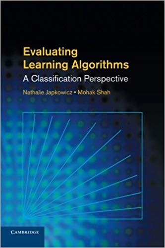
• This book, 4.6 stars rating on Amazon, delves into the evaluation process, particularly focusing on classification algorithms (Japkowicz and Shah 2011).

• Nathalie Japkowicz previously served as a professor at the University of Ottawa and is currently affiliated with American University in Washington.

• Mohak Shah, who earned his PhD from the University of Ottawa, has held numerous industry roles, including Vice President of AI and Machine Learning at LG Electronics.

Performance Metrics

Confusion Matrix

	Positive (Predicted)	Negative (Predicted)
Positive (Actual)	True positive (TP)	False negative (FN)
Negative (Actual)	False positive (FP)	True negative (TN)

• In statistical analysis, False Positives (FP) are commonly referred to as Type I errors, and False Negatives (FN) are known as Type II errors.

• The confusion matrix encapsulates all essential information required to assess the performance of a classification model.

• While the confusion matrix provides a comprehensive view, more concise metrics such as accuracy, precision, recall, and the F\(_1\) score are often more intuitive and practical for summarizing model performance.

A confusion matrix is a table summarizing the performance of a classification algorithm (here for a binary classification task).

Confusion Matrix

Given a test set with \(N\) examples and a classifier \(h(x):\)

\[ C_{i,j} = \sum_{k = 1}^N [y_k = i \wedge h(x_k) = j] \]

Where \(C\) is \(l \times l\) matrix, for a dataset with \(l\) classes.

A confusion matrix \(C\) is defined such that each element \(C_{i,j}\) represents the count of observations actually belonging to class \(i\) but predicted to belong to class \(j\).

Confusion Matrix

• The total number of examples of the (actual) class \(i\) is \[ C_{i \cdot} = \sum_{j=1}^l C_{i,j} \]

• The total number of examples assigned to the (predicted) class \(j\) by classifier \(h\) is \[ C_{\cdot j} = \sum_{i=1}^l C_{i,j} \]

Confusion Matrix

• Terms on the diagonal denote the total number of examples classified correctly by classifier \(h\). Hence, the number of correctly classified examples is \[ \sum_{i=1}^l C_{i,i} \]

• Non-diagonal terms represent misclassifications.

Considers a deterministic classification and symmetric loss.

Confusion Matrix - Multi-Class

To evaluate performance in a multi-class setting, one typically derives “one-vs-all” metrics for each class from the confusion matrix. These metrics are then averaged using specific weighting schemes.

Confusion Matrix - Multi-Class

Using data from the 20 newsgroups text dataset from scikit-learn.org.

Confusion Matrix - True Positive

comp.graphics is the true class (\(i\)).

Confusion Matrix - False Positive

comp.graphics is the true class (\(i\)).

Confusion Matrix - False Negative

comp.graphics is the true class (\(i\)).

Confusion Matrix - True Negative

comp.graphics is the true class (\(i\)).

Confusion Matrix - Multi-Class

comp.graphics is the true class (\(i\)).

Multi-Class

To evaluate performance in a multi-class setting, one typically derives “one-vs-all” metrics for each class from the confusion matrix. These metrics are then averaged using specific weighting schemes.

• True Positives (\(\mathrm{TP}_i\)): Diagonal entry \(C_{i,i}\).
• False Positives (\(\mathrm{FP}_i\)): Sum of column \(i\) excluding \(C_{i,i}\).
• False Negatives (\(\mathrm{FN}_i\)): Sum of row \(i\) excluding \(C_{i,i}\) .
• True Negatives (\(\mathrm{TN}_i\)): \(N - (\mathrm{TP}_i + \mathrm{FP}_i + \mathrm{FN}_i)\)

Multi-Class

To evaluate performance in a multi-class setting, one typically derives “one-vs-all” metrics for each class from the confusion matrix. These metrics are then averaged using specific weighting schemes.

• \(\mathrm{TP}_i = C_{i,i}\).
• \(\mathrm{FP}_i = \sum_{k \ne i} C_{k,i}\).
• \(\mathrm{FN}_i = \sum_{k \ne i} C_{i,k}\).
• \(\mathrm{TN}_i = \sum_{j \ne i} \sum_{k \ne i} C_{j,k}\).

sklearn.metrics.confusion_matrix

from sklearn.metrics import confusion_matrix

y_actual = [0, 0, 0, 1, 1, 1, 1, 1, 1, 1]
y_pred   = [0, 1, 1, 0, 0, 0, 1, 1, 1, 1]

confusion_matrix(y_actual,y_pred)

array([[1, 2],
       [3, 4]])

tn, fp, fn, tp = confusion_matrix(y_actual, y_pred).ravel()
(tn, fp, fn, tp)

(1, 2, 3, 4)

Perfect Prediction

y_actual = [0, 1, 0, 0, 1, 1, 1, 0, 1, 1]
y_pred   = [0, 1, 0, 0, 1, 1, 1, 0, 1, 1]

confusion_matrix(y_actual,y_pred)

array([[4, 0],
       [0, 6]])

tn, fp, fn, tp = confusion_matrix(y_actual, y_pred).ravel()    
(tn, fp, fn, tp)

(4, 0, 0, 6)

When an algorithm achieves perfect classification accuracy, all non-zero values in the confusion matrix appear exclusively along its diagonal.

All off-diagonal entries, which represent misclassifications, will be zero.

Confusion Matrix - Multiple Classes

from sklearn.datasets import load_digits

import numpy as np
np.random.seed(42)

digits = load_digits()

X = digits.data
y = digits.target

from sklearn.model_selection import train_test_split

X_train, X_test, y_train, y_test = train_test_split(X, y, test_size=0.1)

from sklearn.preprocessing import StandardScaler

scaler = StandardScaler()
X_train = scaler.fit_transform(X_train)

from sklearn.linear_model import LogisticRegression
from sklearn.multiclass import OneVsRestClassifier

clf = OneVsRestClassifier(LogisticRegression())

clf = clf.fit(X_train, y_train)

import matplotlib.pyplot as plt
from sklearn.metrics import ConfusionMatrixDisplay

X_test = scaler.transform(X_test)
y_pred = clf.predict(X_test)

ConfusionMatrixDisplay.from_predictions(y_test, y_pred)
plt.show()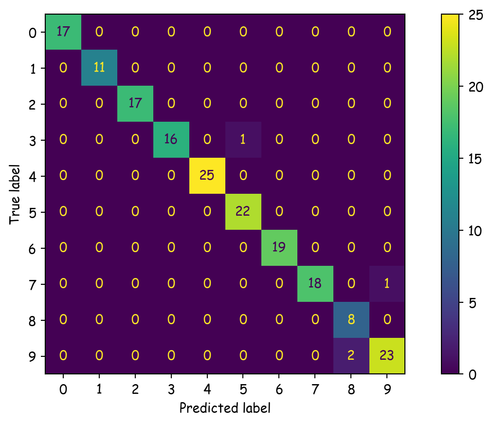

The image displays a heatmap of the confusion matrix for the digit classification task. This task, a multiclass classification problem, was addressed using OneVsRestClassifier and LogisticRegression.

The confusion matrix summarizes the predictions made on the test set, which is a subset of the data that was neither used for training nor for preprocessing with StandardScaler.

The confusion matrix encapsulates all the results from applying the classifier to the test set. However, to summarize this information more succinctly, we often refer to performance metrics.

Confusion matrix for the digits example presented in the previous lecture.

Visualizing errors

mask = (y_test == 9) & (y_pred == 8)

X_9_as_8 = X_test[mask]

y_9_as_8 = y_test[mask]

import numpy as np
np.random.seed(42)

from sklearn.datasets import load_digits
digits = load_digits()

X = digits.data
y = digits.target

from sklearn.model_selection import train_test_split

X_train, X_test, y_train, y_test = train_test_split(X, y, test_size=0.1)

from sklearn.preprocessing import StandardScaler

scaler = StandardScaler()
X_train = scaler.fit_transform(X_train)

from sklearn.linear_model import LogisticRegression
from sklearn.multiclass import OneVsRestClassifier

clf = OneVsRestClassifier(LogisticRegression())

clf = clf.fit(X_train, y_train)

X_test = scaler.transform(X_test)
y_pred = clf.predict(X_test)

mask = (y_test == 9) & (y_pred == 8)

X_9_as_8 = X_test[mask]

y_9_as_8 = y_test[mask]

import matplotlib.pyplot as plt

plt.figure(figsize=(4,2))

for index, (image, label) in enumerate(zip(X_9_as_8, y_9_as_8)):
    plt.subplot(1, len(X_9_as_8), index + 1)
    plt.imshow(np.reshape(image, (8,8)), cmap=plt.cm.gray)
    plt.title(f'y = {label}')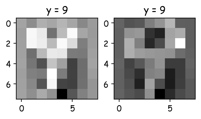

In the confusion matrix on the previous screen, we had seen that there were examples for which the true label was 9, but the prediction was was 8. We can visualize the examples to see if we understand the nature of those errors.

Confusion Matrix - Multiple Classes

It is often preferable to summarize the classifier’s performance with a single metric.

Accuracy

How accurate is this result?

\[ \mathrm{accuracy} = \frac{\mathrm{TP}+\mathrm{TN}}{\mathrm{TP}+\mathrm{TN}+\mathrm{FP}+\mathrm{FN}} = \frac{\mathrm{TP}+\mathrm{TN}}{\mathrm{N}} \]

from sklearn.metrics import accuracy_score

y_actual = [0, 0, 0, 1, 1, 1, 1, 1, 1, 1]
y_pred   = [0, 1, 1, 0, 0, 0, 1, 1, 1, 1]

accuracy_score(y_actual,y_pred)

0.5

Accuracy is the ratio of correctly predicted instances to the total number of predictions.

Accuracy

y_actual = [0, 1, 0, 0, 1, 1, 1, 0, 1, 1]
y_pred   = [1, 0, 1, 1, 0, 0, 0, 1, 0, 0]

accuracy_score(y_actual,y_pred)

0.0

y_actual = [0, 1, 0, 0, 1, 1, 1, 0, 1, 1]
y_pred   = [0, 1, 0, 0, 1, 1, 1, 0, 1, 1]

accuracy_score(y_actual,y_pred)

1.0

Accuracy is a number between 0 (all wrong) and 1 (perfect).

Accuracy can be misleading

y_actual = [0, 0, 0, 0, 1, 1, 0, 0, 0, 0]
y_pred   = [0, 0, 0, 0, 0, 0, 0, 0, 0, 0]

accuracy_score(y_actual,y_pred)

0.8

Accuracy can be misleading in the context of class imbalance, as it disproportionately reflects the performance on the majority class, thereby masking poor performance on the minority class.

As class imbalance increases, the accuracy metric becomes increasingly misleading.

Why is it problematic?

Precision

AKA, positive predictive value (PPV).

\[ \mathrm{precision} = \frac{\mathrm{TP}}{\mathrm{TP}+\mathrm{FP}} \]

from sklearn.metrics import precision_score

y_actual = [0, 0, 0, 1, 1, 1, 1, 1, 1, 1]
y_pred   = [0, 1, 1, 0, 0, 0, 1, 1, 1, 1]

precision_score(y_actual, y_pred)

0.6666666666666666

Precision is the proportion of true positive predictions among all positive predictions.

Precision alone is not enough

y_actual = [0, 0, 0, 1, 1, 1, 1, 1, 1, 1]
y_pred   = [0, 0, 0, 0, 0, 0, 1, 0, 0, 0]

precision_score(y_actual,y_pred)

1.0

An algorithm that makes a small number of high-confidence predictions might achieve a high precision score, but this may not necessarily be useful.

Recall

AKA sensitivity or true positive rate (TPR) \[ \mathrm{recall} = \frac{\mathrm{TP}}{\mathrm{TP}+\mathrm{FN}} \]

from sklearn.metrics import recall_score

y_actual = [0, 0, 0, 1, 1, 1, 1, 1, 1, 1]
y_pred   = [0, 1, 1, 0, 0, 0, 1, 1, 1, 1]

recall_score(y_actual,y_pred)

0.5714285714285714

Recall is the proportion of true positive instances correctly identified among all actual positive instances.

F\(_1\) score

\[ \begin{align*} F_1~\mathrm{score} &= \frac{2}{\frac{1}{\mathrm{precision}}+\frac{1}{\mathrm{recall}}} = 2 \times \frac{\mathrm{precision}\times\mathrm{recall}}{\mathrm{precision}+\mathrm{recall}} \\ &= \frac{\mathrm{TP}}{\mathrm{FP}+\frac{\mathrm{FN}+\mathrm{FP}}{2}} \end{align*} \]

from sklearn.metrics import f1_score

y_actual = [0, 0, 0, 1, 1, 1, 1, 1, 1, 1]
y_pred   = [0, 1, 1, 0, 0, 0, 1, 1, 1, 1]

f1_score(y_actual,y_pred)

0.6153846153846154

• The harmonic mean places greater emphasis on lower values, while the arithmetic mean treats all values equally.
• Using the harmonic mean ensures that a high score is only achieved when both precision and recall are high, thus providing a more holistic measure of a classifier’s performance in scenarios with imbalanced datasets.
• The F\(_1\) score favors classifiers that achieve a balance between precision and recall.
• Increasing recall often results in a decrease in precision, and vice versa. This phenomenon is known as the precision/recall trade-off.

F\(_1\) is the harmonic mean of precision and recall.

Micro and Macro Averaging

Definition

The class imbablance problem is a scenario where the number of instances in one class significantly outnumbers the instances in other classes.

Models tend to be biased towards the majority class, leading to poor performance on the minority class.

Standard evaluation metrics like accuracy may be misleading in the presence of class imbalance.

Micro Performance Metrics

• Micro performance metrics aggregate the contributions of all instances to compute average performance metrics like precision, recall, or F1 score.
• This approach treats each individual prediction equally, regardless of its class, as it considers the total number of true positives, false positives, and false negatives across all classes.
• Consequently, micro metrics are particularly sensitive to the performance on frequent classes because they are more numerous and thus have a greater influence on the overall metric.

Macro Performance Metrics

• Macro performance metrics compute the performance metric independently for each class and then average these metrics.
• This approach treats each class equally, regardless of its frequency, providing an evaluation that equally considers performance across both frequent and infrequent classes.
• Consequently, macro metrics are less sensitive to the performance on frequent classes.

Multi-Class

When calculating precision, recall, and \(F_1\), one usually compute “one-vs-all” metrics for each class. Then, average them using weighting schemes (macro, micro).

• True Positives (\(\mathrm{TP}_i\)): Diagonal entry \(C_{i,i}\).
• False Positives (\(\mathrm{FP}_i\)): Sum of column \(i\) excluding \(C_{i,i}\).
• False Negatives (\(\mathrm{FN}_i\)): Sum of row \(i\) excluding \(C_{i,i}\) .
• True Negatives (\(\mathrm{TN}_i\)): \(N - (\mathrm{TP}_i + \mathrm{FP}_i + \mathrm{FN}_i)\)

Multi-Class

When calculating precision, recall, and \(F_1\), one usually compute “one-vs-all” metrics for each class. Then, average them using weighting schemes (macro, micro).

• \(\mathrm{TP}_i = C_{i,i}\).
• \(\mathrm{FP}_i = \sum_{k \ne i} C_{k,i}\).
• \(\mathrm{FN}_i = \sum_{k \ne i} C_{i,k}\).
• \(\mathrm{TN}_i = \sum_{j \ne i} \sum_{k \ne i} C_{j,k}\).

Micro/Macro Metrics

from sklearn.metrics import ConfusionMatrixDisplay

# Sample data
y_true = ['Cat'] * 42 + ['Dog'] *  7 + ['Fox'] * 11
y_pred = ['Cat'] * 39 + ['Dog'] *  1 + ['Fox'] *  2 + \
         ['Cat'] *  4 + ['Dog'] *  3 + ['Fox'] *  0 + \
         ['Cat'] *  5 + ['Dog'] *  1 + ['Fox'] *  5

ConfusionMatrixDisplay.from_predictions(y_true, y_pred)

The dataset can be conceptualized as resulting from an image classification task, involving images of cats, dogs, and foxes. Reflecting common trends observed on the internet, images of cats are disproportionately represented, leading to a class imbalance issue.

Micro/Macro Precision

from sklearn.metrics import classification_report, precision_score

print(classification_report(y_true, y_pred), "\n")

print("Micro precision: {:.2f}".format(precision_score(y_true, y_pred, average='micro')))
print("Macro precision: {:.2f}".format(precision_score(y_true, y_pred, average='macro')))

              precision    recall  f1-score   support

         Cat       0.81      0.93      0.87        42
         Dog       0.60      0.43      0.50         7
         Fox       0.71      0.45      0.56        11

    accuracy                           0.78        60
   macro avg       0.71      0.60      0.64        60
weighted avg       0.77      0.78      0.77        60
 

Micro precision: 0.78
Macro precision: 0.71

Micro/Macro Precision

• Macro-average precision is calculated as the mean of the precision scores¹ for each class: \(\frac{0.81 + 0.60 + 0.71}{3} = 0.71\).

• Whereas, the micro-average precision is calculated using the formala, \(\frac{TP}{TP+FP}\) and the data from the entire confusion matrix \(\frac{39+3+5}{39+3+5+9+2+2} = \frac{47}{60} = 0.78\)

The high micro-average precision observed here is primarily due to the high precision and large number of examples in the majority class, Cat. This masks the classifier’s relatively poor performance on the minority classes, Dog and Fox.

In a balanced dataset, both micro-average and macro-average metrics yield similar scores.

However, in an imbalanced dataset, significant disparities in classifier performance between the majority and minority classes will result in divergent micro-average and macro-average scores. Specifically, the classifier tends to underperform on the minority class(es), leading to these discrepancies.

In macro-average metrics, each class contributes equally to the final metric calculation, irrespective of the number of examples it contains. This means that the performance metric for each class are computed independently and then averaged, without considering the proportion of instances that each class represents in the dataset. Consequently, macro-averaging ensures that each class has an equal impact on the overall metric, which can be particularly useful in cases where the class distribution is imbalanced.

1. Therefore, macro-average precision remains unaffected by the varying number of examples across different classes.

Micro/Macro Recall

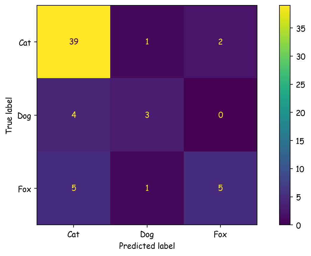
              precision    recall  f1-score   support

         Cat       0.81      0.93      0.87        42
         Dog       0.60      0.43      0.50         7
         Fox       0.71      0.45      0.56        11

    accuracy                           0.78        60
   macro avg       0.71      0.60      0.64        60
weighted avg       0.77      0.78      0.77        60
 

Micro recall: 0.78
Macro recall: 0.60

Micro/Macro Recall

• Macro-average recall is calculated as the mean of the recall scores for each class: \(\frac{0.93 + 0.43 + 0.45}{3} = 0.60\).

• Whereas, the micro-average recall is calculated using the formala, \(\frac{TP}{TP+FN}\) and the data from the entire confusion matrix \(\frac{39+3+5}{39+3+5+3+4+6} = \frac{39}{60} = 0.78\)

Example

Using the 20 newsgroups text dataset from scikit-learn.org.

Comprises around 18,000 newsgroups posts on 20 topics.

## https://scikit-learn.org/stable/auto_examples/text/plot_document_classification_20newsgroups.html

from time import time

## Load Dataset

from sklearn.datasets import fetch_20newsgroups
from sklearn.feature_extraction.text import TfidfVectorizer

categories = [
    "alt.atheism",
    "talk.religion.misc",
    "comp.graphics",
    "sci.space",
]

def size_mb(docs):
    return sum(len(s.encode("utf-8")) for s in docs) / 1e6

def load_dataset(verbose=False, remove=()):
    """Load and vectorize the 20 newsgroups dataset."""

    data_train = fetch_20newsgroups(
        subset="train",
        categories=categories,
        shuffle=True,
        random_state=42,
        remove=remove,
    )

    data_test = fetch_20newsgroups(
        subset="test",
        categories=categories,
        shuffle=True,
        random_state=42,
        remove=remove,
    )

    # order of labels in `target_names` can be different from `categories`
    target_names = data_train.target_names

    # split target in a training set and a test set
    y_train, y_test = data_train.target, data_test.target

    # Extracting features from the training data using a sparse vectorizer
    t0 = time()
    vectorizer = TfidfVectorizer(
        sublinear_tf=True, max_df=0.5, min_df=5, stop_words="english"
    )
    X_train = vectorizer.fit_transform(data_train.data)
    duration_train = time() - t0

    # Extracting features from the test data using the same vectorizer
    t0 = time()
    X_test = vectorizer.transform(data_test.data)
    duration_test = time() - t0

    feature_names = vectorizer.get_feature_names_out()

    if verbose:
        # compute size of loaded data
        data_train_size_mb = size_mb(data_train.data)
        data_test_size_mb = size_mb(data_test.data)

        # print(
        #     f"{len(data_train.data)} documents - "
        #     f"{data_train_size_mb:.2f}MB (training set)"
        # )
        # print(f"{len(data_test.data)} documents - {data_test_size_mb:.2f}MB (test set)")
        # print(f"{len(target_names)} categories")
        # print(
        #     f"vectorize training done in {duration_train:.3f}s "
        #     f"at {data_train_size_mb / duration_train:.3f}MB/s"
        # )
        # print(f"n_samples: {X_train.shape[0]}, n_features: {X_train.shape[1]}")
        # print(
        #     f"vectorize testing done in {duration_test:.3f}s "
        #     f"at {data_test_size_mb / duration_test:.3f}MB/s"
        # )
        # print(f"n_samples: {X_test.shape[0]}, n_features: {X_test.shape[1]}")

    return X_train, X_test, y_train, y_test, feature_names, target_names

X_train, X_test, y_train, y_test, feature_names, target_names = load_dataset(
    verbose=True
)

## Training and Prediction

from sklearn.linear_model import RidgeClassifier

clf = RidgeClassifier(tol=1e-2, solver="sparse_cg")
clf.fit(X_train, y_train)
y_pred = clf.predict(X_test)

## Display the Confusion Matrix

from sklearn.metrics import ConfusionMatrixDisplay

fig, ax = plt.subplots(figsize=(10, 5))
ConfusionMatrixDisplay.from_predictions(y_test, y_pred, ax=ax)
ax.xaxis.set_ticklabels(target_names)
ax.yaxis.set_ticklabels(target_names)
_ = ax.set_title(
    f"Confusion Matrix for {clf.__class__.__name__}"
)

Example

Example

cm = confusion_matrix(y_test, y_pred)

TP, FP, FN, TN

def true_positive(cm, i):
    return cm[i,i] # diagonal entry i,i

def false_positive(cm, i):
    return np.sum(cm[:, i]) - cm[i,i] # col - TP_i

def false_negative(cm, i):
    return np.sum(cm[i, :]) - cm[i,i] # row - TP_i

def true_negative(cm, i):
  N = cm.sum()
  TP = true_positive(cm, i)
  FP = false_positive(cm, i)
  FN = false_negative(cm, i)
  return N - (TP + FP + FN)

Precision

def precision_micro(cm):
    _, l = cm.shape
    tp = fp = 0
    for i in range(l):
        tp += true_positive(cm, i)
        fp += false_positive(cm, i)
    return tp / (tp+fp)

def precision_macro(cm):
    _, l = cm.shape
    precision = 0
    for i in range(l):
        tp = true_positive(cm, i)
        fp = false_positive(cm, i)
        precision += tp/(tp+fp)
    return precision/l

Precision Micro Average

\[ \frac{(258+380+371+199)}{(258+380+371+199)+(40+38+22+45)} \] where

• 40 = 2 + 1 + 37
• 38 = 7 + 22 + 9
• 22 = 12 + 4 + 6
• 45 = 42 + 3 + 0

89.28307465 %

Precision Macro Average

• \(\mathrm{Precision}_0 = \frac{258}{258+(2+1+37)} = 0.8657718121\)
• \(\mathrm{Precision}_1 = \frac{380}{380+(7+22+9)} = 0.9090909091\)
• \(\mathrm{Precision}_2 = \frac{371}{371+(12+4+6)} = 0.9440203562\)
• \(\mathrm{Precision}_3 = \frac{199}{199+(42+3+0)} = 0.8155737705\)

\(\mathrm{Precision}_3 = \frac{0.8657718121 + 0.9090909091 + 0.9440203562 + 0.8155737705}{4}\)

88.3614212 %

Recall

def recall_micro(cm):
    _, l = cm.shape
    tp = fn = 0
    for i in range(l):
        tp += true_positive(cm, i)
        fn += false_negative(cm, i)
    return tp / (tp+fn)

def recall_macro(cm):
    _, l = cm.shape
    recall = 0
    for i in range(l):
        tp = true_positive(cm, i)
        fn = false_negative(cm, i)
        recall += tp / (tp+fn)
    return recall/l

Micro/Macro Metrics (Medical Data)

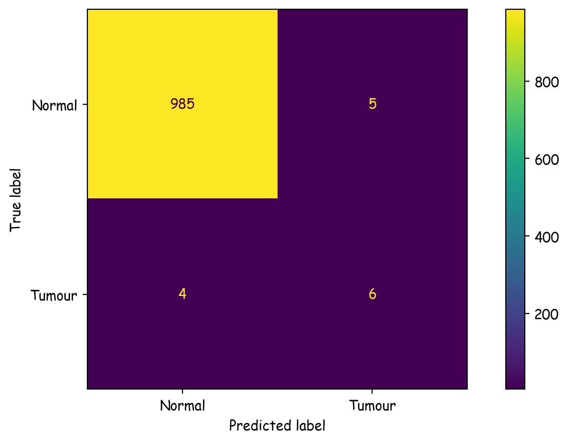
Consider a medical dataset, such as those involving diagnostic tests or imaging, comprising 990 normal samples and 10 abnormal (tumor) samples. This represents the ground truth.

Micro/macro metrics (medical data)

              precision    recall  f1-score   support

      Normal       1.00      0.99      1.00       990
      Tumour       0.55      0.60      0.57        10

    accuracy                           0.99      1000
   macro avg       0.77      0.80      0.78      1000
weighted avg       0.99      0.99      0.99      1000
 

Micro precision: 0.99
Macro precision: 0.77


Micro recall: 0.99
Macro recall: 0.80

The precision for the Tumour class is low. However, due to the small sample size, this does not significantly impact the micro-averaged precision.

Precision-Recall Trade-Off

Hand-Written Digits (Revisited)

Loading the dataset

import numpy as np
np.random.seed(42)

from sklearn.datasets import fetch_openml

digits = fetch_openml('mnist_784', as_frame=False)
X, y = digits.data, digits.target

Plotting the first five examples

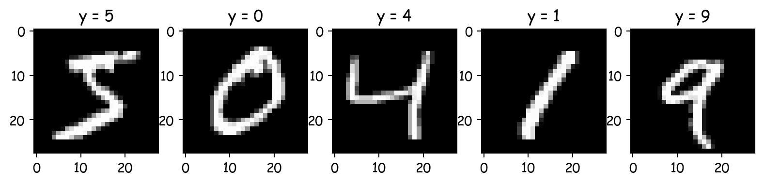
These images have dimensions of \(28 \times 28\) pixels.

Creating a Binary Classification Task

# Creating a binary classification task (one vs the rest)

some_digit = X[0]
some_digit_y = y[0]

y = (y == some_digit_y)
y

array([ True, False, False, ..., False,  True, False])

# Creating the training and test sets
from sklearn.model_selection import train_test_split

X_train, X_test, y_train, y_test = train_test_split(X, y, test_size=0.1)

SGDClassifier

from sklearn.linear_model import SGDClassifier

clf = SGDClassifier()
clf.fit(X_train, y_train)

clf.predict(X[0:5]) # small sanity check

array([ True, False, False, False, False])

The SGDClassifier is a linear classifier that utilizes stochastic gradient descent (SGD) for training. Compared to LogisticRegression, it can offer faster training times, particularly for large datasets. Additionally, SGDClassifier allows for the adjustment of the decision threshold in subsequent examples.

Performance

from sklearn.metrics import accuracy_score

y_pred = clf.predict(X_test)

accuracy_score(y_test, y_pred)

0.9572857142857143

Wow!

Not so Fast

from sklearn.dummy import DummyClassifier

dummy_clf = DummyClassifier()

dummy_clf.fit(X_train, y_train)

y_pred = dummy_clf.predict(X_test)

accuracy_score(y_test, y_pred)

0.906

Why is the accuracy so high despite this classifier ignoring the input data?

The high accuracy is attributed to the class distribution within the dataset. Approximately 10% of the samples correspond to the digit ‘5’, which is the positive class in our binary classification task. Consequently, about 90% of the samples are ‘not 5’ and belong to the negative class. Since the DummyClassifier always predicts the majority class, its accuracy is expected to be around 90%.

This underscores the point that accuracy is often not the best metric, particularly when dealing with imbalanced datasets.

The DummyClassifier in scikit-learn generates predictions without considering the input features. By default, it consistently predicts the most frequent class label in the training data. It is a simple baseline classifier.

Precision-Recall Trade-Off

Attribution: Géron (2022) Figure 3.4

Precision-Recall Trade-Off

from sklearn.model_selection import cross_val_predict
y_scores = cross_val_predict(clf, X_train, y_train, cv=3, method="decision_function")

from sklearn.metrics import precision_recall_curve

precisions, recalls, thresholds = precision_recall_curve(y_train, y_scores)

threshold = 3000

plt.figure(figsize=(8, 4))  # extra code – it's not needed, just formatting
plt.plot(thresholds, precisions[:-1], "b--", label="Precision", linewidth=2)
plt.plot(thresholds, recalls[:-1], "g-", label="Recall", linewidth=2)
plt.vlines(threshold, 0, 1.0, "k", "dotted", label="threshold")

# extra code – this section just beautifies and saves Figure 3–5
idx = (thresholds >= threshold).argmax()  # first index ≥ threshold
plt.plot(thresholds[idx], precisions[idx], "bo")
plt.plot(thresholds[idx], recalls[idx], "go")
plt.axis([-50000, 50000, 0, 1])
plt.grid()
plt.xlabel("Threshold")
plt.legend(loc="center right")

plt.show()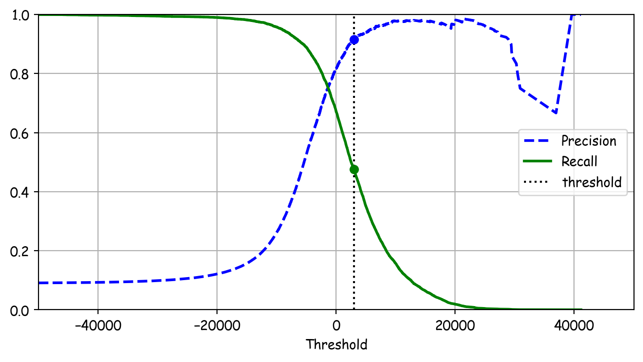

As the decision threshold decreases, a higher number of examples are predicted as positive, potentially leading the classifier to eventually label all instances as positive.

Conversely, as the decision threshold increases, fewer examples are classified as positive, which may result in the classifier predicting no positive instances at all.

For certain applications, a classifier with high precision is essential. For example, consider a scenario where each prediction necessitates a costly laboratory experiment to verify its accuracy, such as in a pharmaceutical company aiming to discover new drugs. Here, the classifier predicts whether a compound is active. Given the high cost of experiments to validate candidates, the company would prioritize focusing on the most promising compounds first.

In contrast, consider a scenario involving cancer screening, such as using mammograms to detect breast cancer. In this case, it may be preferable to lower the decision threshold, thereby increasing the number of false-positive predictions. Although this approach results in more patients undergoing additional tests, such as biopsies, it can potentially save more lives by ensuring that fewer cases of cancer go undetected.

SGDClassifier is used because it allows to vary the decision treshold (boundary) to produce a plot illustrating the precision-recall tradeoff. (Géron 2022) 03_classification.ipynb.

Precision/Recall Curve

import matplotlib.patches as patches  # extra code – for the curved arrow

plt.figure(figsize=(5, 5))  # extra code – not needed, just formatting

plt.plot(recalls, precisions, linewidth=2, label="Precision/Recall Curve")

# extra code – just beautifies and saves Figure 3–6
plt.plot([recalls[idx], recalls[idx]], [0., precisions[idx]], "k:")
plt.plot([0.0, recalls[idx]], [precisions[idx], precisions[idx]], "k:")
plt.plot([recalls[idx]], [precisions[idx]], "ko",
         label="Point at threshold 3,000")
plt.gca().add_patch(patches.FancyArrowPatch(
    (0.79, 0.60), (0.61, 0.78),
    connectionstyle="arc3,rad=.2",
    arrowstyle="Simple, tail_width=1.5, head_width=8, head_length=10",
    color="#444444"))
plt.text(0.56, 0.62, "Higher\nthreshold", color="#333333")
plt.xlabel("Recall")
plt.ylabel("Precision")
plt.axis([0, 1, 0, 1])
plt.grid()
plt.legend(loc="lower left")

plt.show()

(Géron 2022) 03_classification.ipynb.

ROC Curve

ROC Curve

Receiver Operating Characteristics (ROC) curve

• True positive rate (TPR) against false positive rate (FPR)
• An ideal classifier has TPR close to 1.0 and FPR close to 0.0
• \(\mathrm{TPR} = \frac{\mathrm{TP}}{\mathrm{TP}+\mathrm{FN}}\) (recall, sensitivity)
• TPR approaches one when the number of false negative predictions is low
• \(\mathrm{FPR} = \frac{\mathrm{FP}}{\mathrm{FP}+\mathrm{TN}}\) (aka~[1-specificity])
• FPR approaches zero when the number of false positive is low

ROC (Receiver Operating Characteristic) curves are popular in machine learning and statistics for several reasons:

1. Comprehensive Performance Evaluation: ROC curves provide a visual representation of a classifier’s performance across all possible thresholds. By plotting the True Positive Rate (TPR) against the False Positive Rate (FPR), it allows practitioners to evaluate the trade-off between sensitivity (recall) and specificity.
2. Threshold Independence: Unlike metrics like accuracy, ROC curves evaluate classifier performance without relying on a specific decision threshold. This makes them particularly useful in comparing models across varying thresholds.
3. Area Under the Curve (AUC): The Area Under the ROC Curve (AUC) provides a single value summary of the model’s performance. AUC-ROC is often used as a benchmark metric to compare different models, with values ranging from 0.5 (random guessing) to 1.0 (perfect classification).
4. Broad Applicability: ROC curves can be used for any binary classification task and are easily extended to multiclass problems using techniques like one-vs-rest classification, making them versatile in evaluating classifiers.

ROC Curve

ROC Curve

idx_for_90_precision = (precisions >= 0.90).argmax()
threshold_for_90_precision = thresholds[idx_for_90_precision]
y_train_pred_90 = (y_scores >= threshold_for_90_precision)

from sklearn.metrics import roc_curve

fpr, tpr, thresholds = roc_curve(y_train, y_scores)

idx_for_threshold_at_90 = (thresholds <= threshold_for_90_precision).argmax()
tpr_90, fpr_90 = tpr[idx_for_threshold_at_90], fpr[idx_for_threshold_at_90]

plt.figure(figsize=(5, 5))  # extra code – not needed, just formatting
plt.plot(fpr, tpr, linewidth=2, label="ROC curve")
plt.plot([0, 1], [0, 1], 'k:', label="Random classifier's ROC curve")
plt.plot([fpr_90], [tpr_90], "ko", label="Threshold for 90% precision")

# extra code – just beautifies and saves Figure 3–7
plt.gca().add_patch(patches.FancyArrowPatch(
    (0.20, 0.89), (0.07, 0.70),
    connectionstyle="arc3,rad=.4",
    arrowstyle="Simple, tail_width=1.5, head_width=8, head_length=10",
    color="#444444"))
plt.text(0.12, 0.71, "Higher\nthreshold", color="#333333")
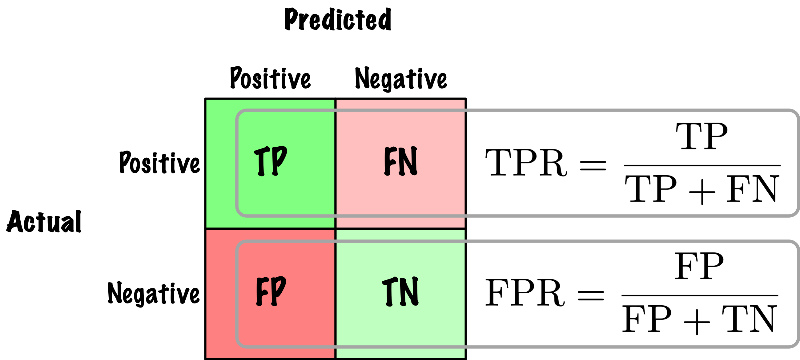
plt.xlabel('False Positive Rate (Fall-Out)')
plt.ylabel('True Positive Rate (Recall)')
plt.grid()
plt.axis([0, 1, 0, 1])
plt.legend(loc="lower right", fontsize=13)

plt.show()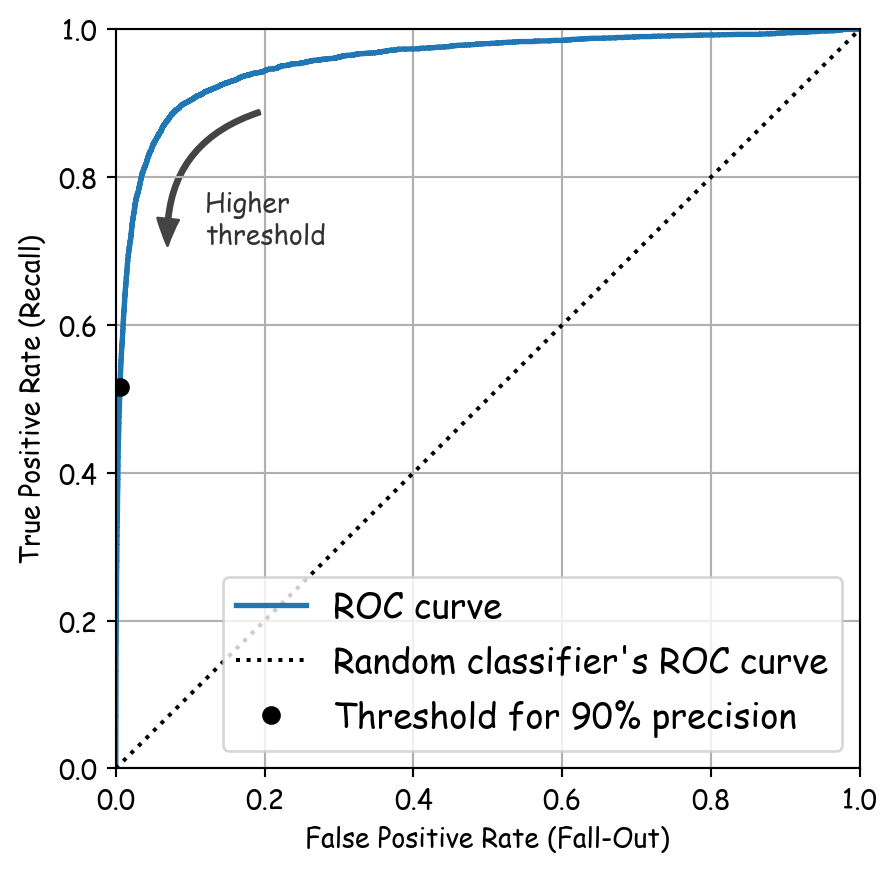

It is common to measure the area under the curve, represented as AUC. Specifically, the area under the ROC curve. This allows to compare

Attribution: 03_classification.ipynb

Dataset - openml

www.openml.org

OpenML is an open platform for sharing datasets, algorithms, and experiments - to learn how to learn better, together.

import numpy as np
np.random.seed(42)

from sklearn.datasets import fetch_openml

diabetes = fetch_openml(name='diabetes', version=1)
print(diabetes.DESCR)

Today’s dataset is the PIMA dataset, which contains 768 instances and 8 numerical attributes. The numerical nature of these attributes facilitates our analysis. Additionally, since the data originates from a published paper, it likely reflects careful data collection, potentially leading to robust results, as the authors would have needed high-quality data to support their publication.

Dataset - openml

Author: Vincent Sigillito

Source: Obtained from UCI

Please cite: UCI citation policy

1. Title: Pima Indians Diabetes Database

2. Sources:

   1. Original owners: National Institute of Diabetes and Digestive and Kidney Diseases
   2. Donor of database: Vincent Sigillito (vgs@aplcen.apl.jhu.edu) Research Center, RMI Group Leader Applied Physics Laboratory The Johns Hopkins University Johns Hopkins Road Laurel, MD 20707 (301) 953-6231
   3. Date received: 9 May 1990

3. Past Usage:

   1. Smith,_J.W., Everhart,_J.E., Dickson,_W.C., Knowler,_W.C., & Johannes,_R.S. (1988). Using the ADAP learning algorithm to forecast the onset of diabetes mellitus. In {it Proceedings of the Symposium on Computer Applications and Medical Care} (pp. 261–265). IEEE Computer Society Press.

      The diagnostic, binary-valued variable investigated is whether the patient shows signs of diabetes according to World Health Organization criteria (i.e., if the 2 hour post-load plasma glucose was at least 200 mg/dl at any survey examination or if found during routine medical care). The population lives near Phoenix, Arizona, USA.

      Results: Their ADAP algorithm makes a real-valued prediction between 0 and 1. This was transformed into a binary decision using a cutoff of 0.448. Using 576 training instances, the sensitivity and specificity of their algorithm was 76% on the remaining 192 instances.

4. Relevant Information: Several constraints were placed on the selection of these instances from a larger database. In particular, all patients here are females at least 21 years old of Pima Indian heritage. ADAP is an adaptive learning routine that generates and executes digital analogs of perceptron-like devices. It is a unique algorithm; see the paper for details.

5. Number of Instances: 768

6. Number of Attributes: 8 plus class

7. For Each Attribute: (all numeric-valued)

   1. Number of times pregnant
   2. Plasma glucose concentration a 2 hours in an oral glucose tolerance test
   3. Diastolic blood pressure (mm Hg)
   4. Triceps skin fold thickness (mm)
   5. 2-Hour serum insulin (mu U/ml)
   6. Body mass index (weight in kg/(height in m)^2)
   7. Diabetes pedigree function
   8. Age (years)
   9. Class variable (0 or 1)

8. Missing Attribute Values: None

9. Class Distribution: (class value 1 is interpreted as “tested positive for diabetes”)

   Class Value Number of instances 0 500 1 268

10. Brief statistical analysis:

    Attribute number: Mean: Standard Deviation:

    1.                 3.8     3.4

    2.               120.9    32.0

    3.                69.1    19.4

    4.                20.5    16.0

    5.                79.8   115.2

    6.                32.0     7.9

    7.                 0.5     0.3

    8.                33.2    11.8

Relabeled values in attribute ‘class’ From: 0 To: tested_negative
From: 1 To: tested_positive

Downloaded from openml.org.

Pima Indians Diabetes Dataset

from sklearn.datasets import fetch_openml

# Load the Pima Indians Diabetes dataset
pima = fetch_openml(name='diabetes', version=1, as_frame=True)

# Extract the features and target
X = pima.data
y = pima.target

# Convert target labels 'tested_negative' and 'tested_positive' to 0 and 1
y = y.map({'tested_negative': 0, 'tested_positive': 1})

# Split the dataset
X_train, X_test, y_train, y_test = train_test_split(X, y, test_size=0.3, random_state=42)

Pima Indians Diabetes Dataset as described in Knowler et al. (1981) [PubMed].

Comparing Multiple Classifiers

from sklearn.linear_model import LogisticRegression
from sklearn.neighbors import KNeighborsClassifier
from sklearn.tree import DecisionTreeClassifier
from sklearn.ensemble import RandomForestClassifier

Comparing Multiple Classifiers

lr = LogisticRegression()
lr.fit(X_train, y_train)

knn = KNeighborsClassifier()
knn.fit(X_train, y_train)

dt = DecisionTreeClassifier()
dt.fit(X_train, y_train)

rf = RandomForestClassifier()
rf.fit(X_train, y_train)

Using the default parameters.

AUC/ROC

from sklearn.metrics import roc_auc_score

y_pred_prob_lr = lr.predict_proba(X_test)[:, 1]
y_pred_prob_knn = knn.predict_proba(X_test)[:, 1]
y_pred_prob_dt = dt.predict_proba(X_test)[:, 1]
y_pred_prob_rf = rf.predict_proba(X_test)[:, 1]

# Compute ROC curves
fpr_lr, tpr_lr, _ = roc_curve(y_test, y_pred_prob_lr)
fpr_knn, tpr_knn, _ = roc_curve(y_test, y_pred_prob_knn)
fpr_dt, tpr_dt, _ = roc_curve(y_test, y_pred_prob_dt)
fpr_rf, tpr_rf, _ = roc_curve(y_test, y_pred_prob_rf)

# Compute AUC scores
auc_lr = roc_auc_score(y_test, y_pred_prob_lr)
auc_knn = roc_auc_score(y_test, y_pred_prob_knn)
auc_dt = roc_auc_score(y_test, y_pred_prob_dt)
auc_rf = roc_auc_score(y_test, y_pred_prob_rf)

# Plot ROC curves
plt.figure(figsize=(5, 5)) # plt.figure()
plt.plot(fpr_lr, tpr_lr, color='blue', label=f'Logistic Regression (AUC = {auc_lr:.2f})')
plt.plot(fpr_knn, tpr_knn, color='green', label=f'K-Nearest Neighbors (AUC = {auc_knn:.2f})')
plt.plot(fpr_dt, tpr_dt, color='orange', label=f'Decision Tree (AUC = {auc_dt:.2f})')
plt.plot(fpr_rf, tpr_rf, color='purple', label=f'Random Forest (AUC = {auc_rf:.2f})')
plt.plot([0, 1], [0, 1], color='red', linestyle='--')  # Diagonal line for random chance
plt.xlim([0.0, 1.0])
plt.ylim([0.0, 1.05])
plt.xlabel('False Positive Rate')
plt.ylabel('True Positive Rate')
plt.title('ROC Curves for Logistic Regression, KNN, Decision Tree, and Random Forest')
plt.legend(loc="lower right")
plt.show()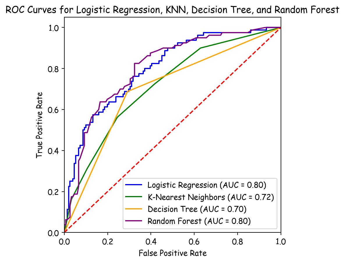

ROC curves provide a visual representation of a classifier’s performance across all possible thresholds. By plotting the True Positive Rate (TPR) against the False Positive Rate (FPR), it allows practitioners to evaluate the trade-off between sensitivity (recall) and specificity.

Unlike metrics like accuracy, ROC curves evaluate classifier performance without relying on a specific decision threshold. This makes them particularly useful in comparing models across varying thresholds.

Implementation: Logistic Regression

Below is our implementation of the logistic regression.

def sigmoid(z):
    """Compute the sigmoid function."""
    return 1 / (1 + np.exp(-z))

def cost_function(theta, X, y):
    """
    Compute the binary cross-entropy cost.
    theta: parameter vector
    X: feature matrix (each row is an example)
    y: true binary labels (0 or 1)
    """
    m = len(y)
    h = sigmoid(X.dot(theta))
    # Add a small epsilon to avoid log(0)
    epsilon = 1e-5
    cost = -(1/m) * np.sum(y * np.log(h + epsilon) + (1 - y) * np.log(1 - h + epsilon))
    return cost

def gradient(theta, X, y):
    """Compute the gradient of the cost with respect to theta."""
    m = len(y)
    h = sigmoid(X.dot(theta))
    return (1/m) * X.T.dot(h - y)

def logistic_regression(X, y, learning_rate=0.1, iterations=1000):
    """
    Train logistic regression using gradient descent.
    Returns the optimized parameter vector theta and the history of cost values.
    """
    m, n = X.shape
    theta = np.zeros(n)
    cost_history = []
    for i in range(iterations):
        theta -= learning_rate * gradient(theta, X, y)
        cost_history.append(cost_function(theta, X, y))
    return theta, cost_history

def predict_probabilities(theta, X):
    """Return predicted probabilities for the positive class."""
    return sigmoid(X.dot(theta))

Implementation: ROC

def compute_roc_curve(y_true, y_scores, thresholds):
    tpr_list, fpr_list = [], []
    for thresh in thresholds:
        # Classify as positive if predicted probability >= threshold
        y_pred = (y_scores >= thresh).astype(int)
        TP = np.sum((y_true == 1) & (y_pred == 1))
        FN = np.sum((y_true == 1) & (y_pred == 0))
        FP = np.sum((y_true == 0) & (y_pred == 1))
        TN = np.sum((y_true == 0) & (y_pred == 0))
        TPR = TP / (TP + FN) if (TP + FN) > 0 else 0
        FPR = FP / (FP + TN) if (FP + TN) > 0 else 0
        tpr_list.append(TPR)
        fpr_list.append(FPR)
    tpr_list.sort()
    fpr_list.sort()
    return np.array(fpr_list), np.array(tpr_list)

Implementation: AUC ROC

def compute_auc(fpr, tpr):
    """
    Compute the Area Under the Curve (AUC) using the trapezoidal rule.
    
    fpr: array of false positive rates
    tpr: array of true positive rates
    """
    return np.trapz(tpr, fpr)

The Trapezoidal Rule (trapz), akin to the Riemann Sum, is a numerical method for approximating the definite integral of a function. By partitioning the area under the curve into trapezoids rather than rectangles, it typically yields a more precise approximation.

Example: Generate Data + Predictions

# Generate synthetic data for binary classification
np.random.seed(0)
m = 100  # number of samples
X = np.random.randn(m, 2)
noise = 0.5 * np.random.randn(m)

# Define labels: a noisy linear combination thresholded at 0
y = (X[:, 0] + X[:, 1] + noise > 0).astype(int)

# Add an intercept term (a column of ones) to X
X_intercept = np.hstack([np.ones((m, 1)), X])

# Train logistic regression model using gradient descent
theta, cost_history = logistic_regression(X_intercept, y, learning_rate=0.1, iterations=1000)

Example: Plot

# Compute predicted probabilities for the positive class
y_probs = predict_probabilities(theta, X_intercept)

# Define a set of threshold values between 0 and 1 (e.g., 100 equally spaced thresholds)
thresholds = np.linspace(0, 1, 100)

# Compute the ROC curve (FPR and TPR for each threshold)
fpr, tpr = compute_roc_curve(y, y_probs, thresholds)
auc_value = compute_auc(fpr, tpr)

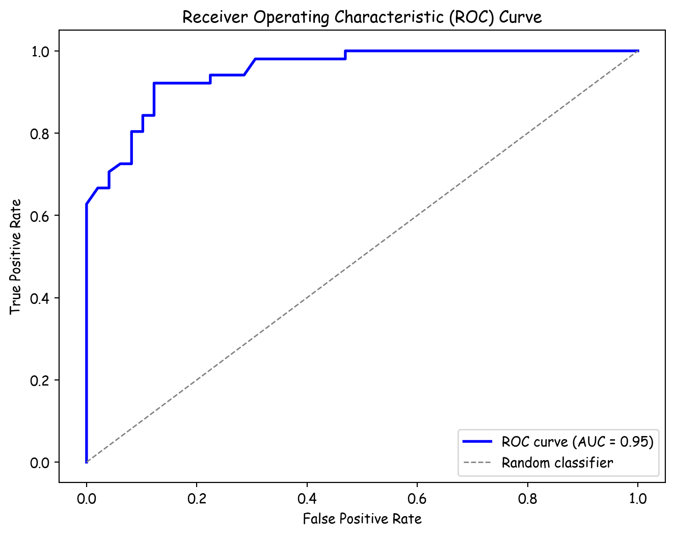
# Plot the ROC curve
plt.figure(figsize=(8, 6))
plt.plot(fpr, tpr, color='blue', lw=2, label='ROC curve (AUC = %0.2f)' % auc_value)
plt.plot([0, 1], [0, 1], color='gray', lw=1, linestyle='--', label='Random classifier')
plt.xlabel('False Positive Rate')
plt.ylabel('True Positive Rate')
plt.title('Receiver Operating Characteristic (ROC) Curve')
plt.legend(loc="lower right")
plt.show()

See Also

• Multiclass Receiver Operating Characteristic (ROC) presents examples of micro- and macro- average curves.

Cross-Validation

Training and test set

Sometimes called holdout method.

• Guideline: Typically, allocate 80% of your dataset for training and reserve the remaining 20% for testing.

• Training Set: This subset of data is utilized to train your model.

• Test Set: This is an independent subset used exclusively at the final stage to assess the model’s performance.

Common Training and Testing Ratios

1. 80:20 Split:
   • Training Set: 80% of the data
   • Testing Set: 20% of the data
   • This is a widely used default split that provides a balance between having enough data to train the model and enough data to evaluate its performance.
2. 90:10 Split:
   • Training Set: 90% of the data
   • Testing Set: 10% of the data
   • This split might be used when the dataset is very large, ensuring a substantial amount of data for training while still having a decent-sized test set.

Considerations for Choosing the Split Ratio

1. Dataset Size:
   • For large datasets, a smaller proportion can be reserved for testing (e.g., 90:10) since even 10% of a large dataset can provide a robust evaluation.
2. Model Complexity:
   • Complex models with many parameters may require more training data to avoid overfitting, suggesting a larger training set.
3. Validation Set:
   • See discussion below.
4. Imbalanced Datasets:
   • For imbalanced datasets, it’s essential to ensure that both the training and testing sets represent the class distribution adequately. Stratified sampling can be used to maintain the class proportions in both sets.

Training and test set

Training Error:

• Generally tends to be low
• Achieved by optimizing learning algorithms to minimize error through parameter adjustments (e.g., weights)

Definition

Generalization Error: The error rate observed when the model is evaluated on new, unseen data.

Prologue

Summary

• Examined classification model evaluation techniques, focusing on confusion matrices and key metrics: accuracy, precision, recall, and \(F_1\) score.
• Addressed the limitations of accuracy in imbalanced datasets, introducing micro and macro averaging techniques.
• Explored the precision-recall trade-off and ROC analysis, including the area under the curve (AUC).
• Provided practical insights through Python implementations.

Next lecture

• Cross-evaluation

References

Géron, Aurélien. 2022. Hands-on Machine Learning with Scikit-Learn, Keras, and TensorFlow. 3rd ed. O’Reilly Media, Inc.

Japkowicz, Nathalie, and Mohak Shah. 2011. Evaluating Learning Algorithms: A Classification Perspective. Cambridge: Cambridge University Press.

Knowler, William C., David J. Pettitt, Peter J. Savage, and Peter H. Bennett. 1981. “Diabetes Incidence in Pima Indians: Contributions of Obesity and Parental Diabetes.” American Journal of Epidemiology 113 2: 144–56. https://api.semanticscholar.org/CorpusID:25209675.

Rafi, Abdul Muntakim, Brett Kiyota, Nozomu Yachie, and Carl G de Boer. 2025. “Detecting and avoiding homology-based data leakage in genome-trained sequence models.” https://doi.org/10.1101/2025.01.22.634321.

Sokolova, Marina, and Guy Lapalme. 2009. “A systematic analysis of performance measures for classification tasks.” Information Processing and Management 45 (4): 427–37. https://doi.org/10.1016/j.ipm.2009.03.002.

Walsh, Ian, Dmytro Fishman, Dario Garcia-Gasulla, Tiina Titma, Gianluca Pollastri, ELIXIR Machine Learning Focus Group, Emidio Capriotti, et al. 2021. “DOME: recommendations for supervised machine learning validation in biology.” Nature Methods 18 (10): 1122–27. https://doi.org/10.1038/s41592-021-01205-4.

Whalen, Sean, Jacob Schreiber, William S. Noble, and Katherine S. Pollard. 2022. “Navigating the pitfalls of applying machine learning in genomics.” Nature Reviews Genetics 23 (3): 169–81. https://doi.org/10.1038/s41576-021-00434-9.

Marcel Turcotte

Marcel.Turcotte@uOttawa.ca

School of Electrical Engineering and Computer Science (EECS)

University of Ottawa