Performance Evaluation

CSI 5180 - Machine Learning for Bioinformatics

Marcel Turcotte

Version: Feb 27, 2025 10:24

Preamble

Quote of the Day (1/2)

Robert F. Kennedy Jr. on Wikipedia:

• “In December 2024, more than 75 Nobel Laureates urged the U.S. Senate to oppose Kennedy’s nomination, saying he would ‘put the public’s health in jeopardy.’”
• “As of January 9, 2025, over 17,000 doctors, who are members of Committee to Protect Health Care, signed an open letter urging the U.S. Senate to oppose Kennedy’s nomination, arguing that Kennedy has spent decades undermining public confidence in vaccines, spreading false claims and conspiracy theories, that he is a danger to national healthcare, and that he lacks the qualifications to lead the Department of Health and Human Services.”
• Gregg Gonsalves, an epidemiologist at the Yale School of Public Health, said putting Kennedy in charge of a health agency would be like “putting a flat earther in charge of NASA.”
• As of January 24, 2025, more than 80 organizations had voiced their opposition to Kennedy’s nomination.

Quote of the Day (2/2)

Nature News, February 6, 2025

“I think writing reviews is becoming obsolete.”

Introducing (OpenAI) deep research

Summary

This lecture covers performance evaluation in machine learning with an emphasis on bioinformatics applications. It details cross-validation methods (including k-fold, group, and leave-one-out), discusses the implications of data leakage and class imbalance, and illustrates hyperparameter tuning via grid and randomized search. Practical Python examples demonstrate evaluation metrics, the curse of dimensionality, and the challenges of applying ML in biological settings.

Learning Outcomes

• Understand and implement k-fold and group cross-validation to assess model generalization.
• Identify and mitigate common pitfalls such as data leakage and class imbalance.
• Apply hyperparameter tuning techniques (grid and randomized search) to optimize model performance.
• Analyze the impact of the curse of dimensionality on distance metrics and classifier reliability.

Definition

Cross-validation is a method used to evaluate and improve the performance of machine learning models.

It involves partitioning the dataset into multiple subsets, training distinct models on some subsets while validating them on the remaining ones.

k-Fold Cross-Validation

1. Dataset Partitioning: Divide the dataset into \(k\) equally sized folds (subsets).

2. Training and Validation Process:

   • For each iteration/fold:
     • Instantiate a new model.
     • Designate one fold as the validation set and the remaining \(k\)-1 folds as the training set.
     • Performance Evaluation: Assess the model’s performance in each iteration, yielding \(k\) distinct performance metrics.

3. Result Aggregation: Compute summary statistics from the \(k\) performance metrics.

Common choices for the value of \(k\) are 3, 5, 7, and 10.

k-Fold Cross-Validation

import matplotlib.pyplot as plt
import numpy as np

def plot_k_fold_cross_validation(k):
    # Create a figure and axis
    fig, ax = plt.subplots()

    plt.rcParams["font.family"] = "Comic Sans MS"

    # Generate k x k matrix with ones for training, zeros for validation
    matrix = np.ones((k, k))
    
    # Make the diagonal elements different (indicating the validation sets)
    np.fill_diagonal(matrix, 0)

    # Display the matrix as an image
    ax.imshow(matrix, cmap='binary', interpolation='none')

    # Annotate the figure with 'Train' and 'Validation'
    for i in range(k):
        for j in range(k):
            if i == j:
                text = 'Validation'
            else:
                text = 'Train'
            ax.text(j, i, text, ha="center", va="center", color="black" if i == j else "white")

    # Set axis labels and title
    ax.set_xticks(np.arange(k))
    ax.set_yticks(np.arange(k))
    ax.set_xticklabels([f"Fold {i+1}" for i in range(k)])
    ax.set_yticklabels([f"Iteration {i+1}" for i in range(k)])
    plt.title(f'{k}-Fold Cross-validation')

    # Turn grid on and show plot
    ax.grid(False)
    plt.show()

3-Fold Cross-validation

plot_k_fold_cross_validation(3)

Each row of the table represents an iteration within the \(k\)-fold cross-validation process, with the number of iterations equating to the number of folds. In each iteration, one fold is designated for validation, while the remaining \(k-1\) folds are utilized for training the model.

With each iteration, \(2/3\) of the dataset is used for training and \(1/3\) for validation.

5-Fold Cross-validation

plot_k_fold_cross_validation(5)

With each iteration, \(4/5\) of the dataset is used for training and \(1/5\) for validation.

Result Aggregation

(Japkowicz and Shah 2011)

However, in the cases in which the size of the overall data at hand is limited, resampling approaches [cross-validation] are utilized that divide the data into training sets and test sets [validation sets] and perform runs over these divisions multiple times. In this case, the confusion matrix entries would be the combined performance of the learning algorithm on the test sets over all such runs (and hence represent the combined performance of classifiers in each run).

Result Aggregation

• In practice, researchers typically report the mean and standard deviation of performance metrics calculated independently for each fold, rather than aggregating confusion matrices.

• This “macro-averaging” technique is prevalent because it considers each fold as an independent evaluation of generalization capability. Furthermore, it facilitates the assessment of variability across folds, which is crucial for evaluating stability.

See also: stats.stackexchange.com and datascience.stackexchange.com.

True or False

• In \(k\)-fold cross-validation, each example is used for validation exactly once.

More Reliable Model Evaluation

• More reliable estimate of model performance compared to a single train-test split.
• Reduces the variability associated with a single split, leading to a more stable and unbiased evaluation.
• For large values of \(k\)¹, consider the average, variance, and confidence interval.

1. 10-fold cross-validation.

Better Generalization

• Helps in assessing how the model generalizes to an independent dataset.
• It ensures that the model’s performance is not overly optimistic or pessimistic by averaging results over multiple folds.

Efficient Use of Data

• Particularly beneficial for small datasets, cross-validation ensures that every data point is used for both training and validation.
• This maximizes the use of available data, leading to more accurate and reliable model training.

Some examples are more informative for learning algorithms, sometimes those near the decision boundary.

Case Study

Definition

The curse of dimensionality refers to the exponential increase in a space’s volume with each added dimension, which causes data to become sparse and renders distance metrics, sampling, and traditional algorithms less effective.

(Altman and Krzywinski 2018)

Example

Curse of Dimensionality

import seaborn as sns
from scipy.spatial.distance import pdist, squareform

# Set random seed for reproducibility
np.random.seed(42)

N = 100
dimensions = [2, 100, 1000]

# Create a figure with one subplot per dimension
fig, axes = plt.subplots(1, len(dimensions), figsize=(15, 5))

for ax, D in zip(axes, dimensions):
    # Generate random data: N examples in D dimensions
    X = np.random.uniform(0, 1, (N, D))
    
    # Compute all pairwise Euclidean distances
    # pdist returns a condensed distance matrix; squareform converts it to a symmetric square matrix.
    dist_matrix = squareform(pdist(X, metric='euclidean'))
    
    # For each example, compute the average distance to all other examples.
    # The diagonal is zero, so we sum the distances along each row and divide by (N-1).
    avg_distances = dist_matrix.sum(axis=1) / (N - 1)
    
    # Plot a histogram of the average distances using Seaborn.
    sns.histplot(avg_distances, bins=12, kde=True, ax=ax)
    ax.set_title(f'D = {D}')
    ax.set_xlabel('Average distance')
    ax.set_ylabel('Count')

plt.tight_layout()
plt.show()

k-Nearest Neighbors

The \(k\)-nearest neighbor (\(k\)-NN) algorithm is a simple, non-parametric, instance-based learning method used for classification and regression. It classifies a data point based on the majority label of its \(k\) nearest neighbors in the feature space, where \(k\) is a user-defined constant. Distance metrics like Euclidean distance are commonly used to determine the nearest neighbors.

A non-parametric algorithm does not make any assumptions about the underlying data distribution and does not learn a fixed set of parameters or a model during the training phase. Instead, it relies directly on the training data to make decisions at the time of classification or regression, making it flexible and adaptive to various data shapes but potentially computationally expensive at prediction time.

In scikit-learn, several models are commonly used for regression tasks. Here are some of the main models:

1. Linear Regression (LinearRegression):
   • A simple linear approach that models the relationship between the independent variables and the dependent variable by fitting a linear equation to the observed data.
2. Support Vector Regression (SVR):
   • An extension of Support Vector Machines (SVM) for regression tasks, which tries to fit the best line within a specified margin of tolerance.
3. Decision Tree Regression (DecisionTreeRegressor):
   • Uses decision trees to model the relationship between the input features and the target variable by recursively splitting the data into subsets.
4. Random Forest Regression (RandomForestRegressor):
   • An ensemble method that uses multiple decision trees to improve predictive accuracy and control overfitting.
5. Gradient Boosting Regression (GradientBoostingRegressor):
   • Another ensemble method that builds sequential decision trees, where each tree corrects the errors of the previous one.
6. K-Nearest Neighbors Regression (KNeighborsRegressor):
   • A non-parametric method that predicts the target variable based on the average of the k-nearest neighbors in the feature space.

These models offer a range of approaches to handle different types of regression problems, each with its own strengths and suitable applications.

See: Nearest Neighbors Classification, KNeighborsClassifier, examples, KNeighborsRegressor, exemples from scikit-learn.

Data

def generate_dataset(N, D):

    """
    Generate a dataset with N examples in D dimensions.
    Each feature is drawn uniformly from [0,1], and the label is 1
    if the sum of features exceeds D/2, and 0 otherwise.
    """

    X = np.random.uniform(0, 1, size=(N, D))
    y = (np.sum(X, axis=1) > (D / 2)).astype(int)
    return X, y

Evaluation

from sklearn.linear_model import LogisticRegression
from sklearn.neighbors import KNeighborsClassifier
from sklearn.dummy import DummyClassifier
from sklearn.model_selection import StratifiedKFold, cross_val_score
import warnings

# Suppress convergence and other warnings
warnings.filterwarnings("ignore")

def evaluate_classifiers_for_N(N, dimensions, cv, k_values):
    print(f"Results for N = {N}")
    for D in dimensions:
        X, y = generate_dataset(N, D)
        
        # Evaluate Dummy Classifier
        dummy = DummyClassifier(strategy='most_frequent')
        scores_dummy = cross_val_score(dummy, X, y, cv=cv, scoring='accuracy')
        
        # Evaluate Logistic Regression
        lr = LogisticRegression(solver='lbfgs', max_iter=1000)
        scores_lr = cross_val_score(lr, X, y, cv=cv, scoring='accuracy')
        
        print(f"  D = {D}:")
        print(f"    Dummy Classifier Accuracy: {scores_dummy.mean():.2f} ± {scores_dummy.std():.2f}")
        print(f"    Logistic Regression Accuracy: {scores_lr.mean():.2f} ± {scores_lr.std():.2f}")
        
        # Evaluate K-Nearest Neighbors for different k values
        for k in k_values:
            knn = KNeighborsClassifier(n_neighbors=k)
            scores_knn = cross_val_score(knn, X, y, cv=cv, scoring='accuracy')
            print(f"    {k}-NN Accuracy: {scores_knn.mean():.2f} ± {scores_knn.std():.2f}")
    print()

N = 100

# N_values = [100, 1000, 10000, 100000]
dimensions = [2, 100, 1000]
k_values = [1, 3, 5, 7, 9, 15, 21]
num_splits = 5

# Set up 10-fold stratified cross-validation
cv = StratifiedKFold(n_splits=num_splits, shuffle=True, random_state=42)

# Evaluate classifiers for each sample size N
evaluate_classifiers_for_N(100, dimensions, cv, k_values)

Results for N = 100
  D = 2:
    Dummy Classifier Accuracy: 0.52 ± 0.02
    Logistic Regression Accuracy: 0.95 ± 0.05
    1-NN Accuracy: 0.96 ± 0.04
    3-NN Accuracy: 0.94 ± 0.06
    5-NN Accuracy: 0.94 ± 0.04
    7-NN Accuracy: 0.94 ± 0.04
    9-NN Accuracy: 0.93 ± 0.05
    15-NN Accuracy: 0.93 ± 0.05
    21-NN Accuracy: 0.96 ± 0.04
  D = 100:
    Dummy Classifier Accuracy: 0.53 ± 0.02
    Logistic Regression Accuracy: 0.79 ± 0.06
    1-NN Accuracy: 0.66 ± 0.07
    3-NN Accuracy: 0.66 ± 0.10
    5-NN Accuracy: 0.80 ± 0.05
    7-NN Accuracy: 0.78 ± 0.02
    9-NN Accuracy: 0.74 ± 0.07
    15-NN Accuracy: 0.78 ± 0.05
    21-NN Accuracy: 0.70 ± 0.10
  D = 1000:
    Dummy Classifier Accuracy: 0.57 ± 0.02
    Logistic Regression Accuracy: 0.60 ± 0.07
    1-NN Accuracy: 0.57 ± 0.04
    3-NN Accuracy: 0.61 ± 0.10
    5-NN Accuracy: 0.61 ± 0.07
    7-NN Accuracy: 0.54 ± 0.11
    9-NN Accuracy: 0.55 ± 0.10
    15-NN Accuracy: 0.59 ± 0.07
    21-NN Accuracy: 0.63 ± 0.02

N = 1000

# Evaluate classifiers for each sample size N
evaluate_classifiers_for_N(1000, dimensions, cv, k_values)

Results for N = 1000
  D = 2:
    Dummy Classifier Accuracy: 0.51 ± 0.00
    Logistic Regression Accuracy: 0.99 ± 0.01
    1-NN Accuracy: 0.98 ± 0.01
    3-NN Accuracy: 0.98 ± 0.01
    5-NN Accuracy: 0.98 ± 0.01
    7-NN Accuracy: 0.98 ± 0.01
    9-NN Accuracy: 0.98 ± 0.01
    15-NN Accuracy: 0.97 ± 0.01
    21-NN Accuracy: 0.97 ± 0.01
  D = 100:
    Dummy Classifier Accuracy: 0.51 ± 0.00
    Logistic Regression Accuracy: 0.92 ± 0.02
    1-NN Accuracy: 0.59 ± 0.02
    3-NN Accuracy: 0.62 ± 0.02
    5-NN Accuracy: 0.64 ± 0.02
    7-NN Accuracy: 0.66 ± 0.02
    9-NN Accuracy: 0.68 ± 0.01
    15-NN Accuracy: 0.72 ± 0.02
    21-NN Accuracy: 0.73 ± 0.02
  D = 1000:
    Dummy Classifier Accuracy: 0.51 ± 0.00
    Logistic Regression Accuracy: 0.71 ± 0.03
    1-NN Accuracy: 0.53 ± 0.03
    3-NN Accuracy: 0.56 ± 0.03
    5-NN Accuracy: 0.55 ± 0.04
    7-NN Accuracy: 0.57 ± 0.04
    9-NN Accuracy: 0.57 ± 0.03
    15-NN Accuracy: 0.58 ± 0.02
    21-NN Accuracy: 0.58 ± 0.03

N = 10000

# Evaluate classifiers for each sample size N
evaluate_classifiers_for_N(10000, dimensions, cv, k_values)

Results for N = 10000
  D = 2:
    Dummy Classifier Accuracy: 0.50 ± 0.00
    Logistic Regression Accuracy: 1.00 ± 0.00
    1-NN Accuracy: 1.00 ± 0.00
    3-NN Accuracy: 0.99 ± 0.00
    5-NN Accuracy: 0.99 ± 0.00
    7-NN Accuracy: 0.99 ± 0.00
    9-NN Accuracy: 0.99 ± 0.00
    15-NN Accuracy: 0.99 ± 0.00
    21-NN Accuracy: 0.99 ± 0.00
  D = 100:
    Dummy Classifier Accuracy: 0.50 ± 0.00
    Logistic Regression Accuracy: 0.99 ± 0.00
    1-NN Accuracy: 0.61 ± 0.01
    3-NN Accuracy: 0.66 ± 0.01
    5-NN Accuracy: 0.68 ± 0.00
    7-NN Accuracy: 0.70 ± 0.01
    9-NN Accuracy: 0.71 ± 0.01
    15-NN Accuracy: 0.75 ± 0.01
    21-NN Accuracy: 0.77 ± 0.00
  D = 1000:
    Dummy Classifier Accuracy: 0.51 ± 0.00
    Logistic Regression Accuracy: 0.94 ± 0.01
    1-NN Accuracy: 0.53 ± 0.02
    3-NN Accuracy: 0.55 ± 0.01
    5-NN Accuracy: 0.56 ± 0.01
    7-NN Accuracy: 0.56 ± 0.01
    9-NN Accuracy: 0.57 ± 0.00
    15-NN Accuracy: 0.58 ± 0.01
    21-NN Accuracy: 0.59 ± 0.01

N = 100000

# Evaluate classifiers for each sample size N
evaluate_classifiers_for_N(100000, dimensions, cv, k_values)

Results for N = 100000
  D = 2:
    Dummy Classifier Accuracy: 0.50 ± 0.00
    Logistic Regression Accuracy: 1.00 ± 0.00
    1-NN Accuracy: 1.00 ± 0.00
    3-NN Accuracy: 1.00 ± 0.00
    5-NN Accuracy: 1.00 ± 0.00
    7-NN Accuracy: 1.00 ± 0.00
    9-NN Accuracy: 1.00 ± 0.00
    15-NN Accuracy: 1.00 ± 0.00
    21-NN Accuracy: 1.00 ± 0.00
  D = 100:
    Dummy Classifier Accuracy: 0.50 ± 0.00
    Logistic Regression Accuracy: 1.00 ± 0.00
    1-NN Accuracy: 0.63 ± 0.00
    3-NN Accuracy: 0.68 ± 0.00
    5-NN Accuracy: 0.71 ± 0.00
    7-NN Accuracy: 0.73 ± 0.00
    9-NN Accuracy: 0.74 ± 0.00
    15-NN Accuracy: 0.78 ± 0.00
    21-NN Accuracy: 0.80 ± 0.00
  D = 1000:
    Dummy Classifier Accuracy: 0.50 ± 0.00
    Logistic Regression Accuracy: 0.99 ± 0.00
    1-NN Accuracy: 0.54 ± 0.00
    3-NN Accuracy: 0.56 ± 0.00
    5-NN Accuracy: 0.57 ± 0.00
    7-NN Accuracy: 0.58 ± 0.00
    9-NN Accuracy: 0.59 ± 0.00
    15-NN Accuracy: 0.61 ± 0.00
    21-NN Accuracy: 0.62 ± 0.00

Hyperparameter Tuning

Dataset - openml

www.openml.org

OpenML is an open platform for sharing datasets, algorithms, and experiments - to learn how to learn better, together.

import numpy as np
np.random.seed(42)

from sklearn.datasets import fetch_openml

diabetes = fetch_openml(name='diabetes', version=1)
print(diabetes.DESCR)

Today’s dataset is the PIMA dataset, which contains 768 instances and 8 numerical attributes. The numerical nature of these attributes facilitates our analysis. Additionally, since the data originates from a published paper, it likely reflects careful data collection, potentially leading to robust results, as the authors would have needed high-quality data to support their publication.

Dataset - openml

Author: Vincent Sigillito

Source: Obtained from UCI

Please cite: UCI citation policy

1. Title: Pima Indians Diabetes Database

2. Sources:

   1. Original owners: National Institute of Diabetes and Digestive and Kidney Diseases
   2. Donor of database: Vincent Sigillito (vgs@aplcen.apl.jhu.edu) Research Center, RMI Group Leader Applied Physics Laboratory The Johns Hopkins University Johns Hopkins Road Laurel, MD 20707 (301) 953-6231
   3. Date received: 9 May 1990

3. Past Usage:

   1. Smith,_J.W., Everhart,_J.E., Dickson,_W.C., Knowler,_W.C., & Johannes,_R.S. (1988). Using the ADAP learning algorithm to forecast the onset of diabetes mellitus. In {it Proceedings of the Symposium on Computer Applications and Medical Care} (pp. 261–265). IEEE Computer Society Press.

      The diagnostic, binary-valued variable investigated is whether the patient shows signs of diabetes according to World Health Organization criteria (i.e., if the 2 hour post-load plasma glucose was at least 200 mg/dl at any survey examination or if found during routine medical care). The population lives near Phoenix, Arizona, USA.

      Results: Their ADAP algorithm makes a real-valued prediction between 0 and 1. This was transformed into a binary decision using a cutoff of 0.448. Using 576 training instances, the sensitivity and specificity of their algorithm was 76% on the remaining 192 instances.

4. Relevant Information: Several constraints were placed on the selection of these instances from a larger database. In particular, all patients here are females at least 21 years old of Pima Indian heritage. ADAP is an adaptive learning routine that generates and executes digital analogs of perceptron-like devices. It is a unique algorithm; see the paper for details.

5. Number of Instances: 768

6. Number of Attributes: 8 plus class

7. For Each Attribute: (all numeric-valued)

   1. Number of times pregnant
   2. Plasma glucose concentration a 2 hours in an oral glucose tolerance test
   3. Diastolic blood pressure (mm Hg)
   4. Triceps skin fold thickness (mm)
   5. 2-Hour serum insulin (mu U/ml)
   6. Body mass index (weight in kg/(height in m)^2)
   7. Diabetes pedigree function
   8. Age (years)
   9. Class variable (0 or 1)

8. Missing Attribute Values: None

9. Class Distribution: (class value 1 is interpreted as “tested positive for diabetes”)

   Class Value Number of instances 0 500 1 268

10. Brief statistical analysis:

    Attribute number: Mean: Standard Deviation:

    1.                 3.8     3.4

    2.               120.9    32.0

    3.                69.1    19.4

    4.                20.5    16.0

    5.                79.8   115.2

    6.                32.0     7.9

    7.                 0.5     0.3

    8.                33.2    11.8

Relabeled values in attribute ‘class’ From: 0 To: tested_negative
From: 1 To: tested_positive

Downloaded from openml.org.

Dataset - return_X_y

fetch_openml returns a Bunch, a DataFrame, or X and y

from sklearn.datasets import fetch_openml

X, y = fetch_openml(name='diabetes', version=1, return_X_y=True)

Mild imbalance (ratio less than 3 or 4)

print(y.value_counts())

class
tested_negative    500
tested_positive    268
Name: count, dtype: int64

Converting the target labels to 0 and 1

y = y.map({'tested_negative': 0, 'tested_positive': 1})

Hyperparameter Tuning

• Commonly used during hyperparameter tuning, allowing for the selection of the best model parameters based on their performance across multiple folds.
• This helps in identifying the optimal configuration that balances bias and variance.

Challenges

• Computational Cost: Requires multiple model trainings.
  • Leave-One-Out (LOO): Extreme case where ( k = N ).
• Class Imbalance: Folds may not represent minority classes.
  • Use Stratified Cross-Validation to maintain class proportions.
• Complexity: Error-prone implementation, especially for nested cross-validation, bootstraps, or integration into larger pipelines.

Leave-one-out cross-validation (LOO-CV) can lead to overoptimistic performance evaluation, particularly in certain contexts.

Here’s why:

1.  **High Variance**: In LOO-CV, each iteration uses almost all the data for training, leaving only one instance for testing. This can result in high variance in the test error across iterations because the model is trained on nearly the full dataset. Since each training set is very similar to the full dataset, it can lead to overly optimistic estimates of generalization error, especially when the dataset is small or the model has high variance (e.g., decision trees or k-nearest neighbors).
2.  **Overfitting**: Since LOO-CV uses nearly the entire dataset for training in each iteration, complex models (especially ones prone to overfitting) can fit very closely to the data, which might result in a low training error but a misleadingly low test error in some cases.
3.  **Limited assessment of generalization**: LOO-CV might not give a reliable estimate of how well the model generalizes to completely unseen data because the difference between the training set and the full dataset is minimal, leading to a smaller gap between training and test performance.

In practice, this can make the evaluation appear more optimistic than it would be with more robust methods like k-fold cross-validation, where the test sets are larger, and the model has less opportunity to overfit the training data.

cross_val_score

from sklearn import tree

clf = tree.DecisionTreeClassifier()

from sklearn.model_selection import cross_val_score    

clf_scores = cross_val_score(clf, X, y, cv=5)

print("\nScores:", clf_scores)
print(f"\nMean: {clf_scores.mean():.2f}")
print(f"\nStandard deviation: {clf_scores.std():.2f}")

Scores: [0.71428571 0.66883117 0.71428571 0.79738562 0.73202614]

Mean: 0.73

Standard deviation: 0.04

As previously discussed, a significant limitation of decision trees is their propensity for overfitting, which leads to high variance when applied to new datasets. This issue is evident in the observed performance variability, with accuracy ranging from 67% to 79%, which is undesirable for achieving robust model generalization.

sklearn.model_selection.cross_val_score, see also cross_validate.

Workflow

The above image implicitly introduces three categories of data subsets: training, validation, and test.

Attribution: Cross-validation: evaluating estimator performance

Workflow - implementation

from sklearn.datasets import fetch_openml

X, y = fetch_openml(name='diabetes', version=1, return_X_y=True)

y = y.map({'tested_negative': 0, 'tested_positive': 1})

from sklearn.model_selection import train_test_split

X_train, X_test, y_train, y_test = train_test_split(X, y, test_size=0.1)

To maintain simplicity in these lecture notes, we have not applied any pre-processing steps.

Definition

A hyperparameter is a configuration external to the model that is set prior to the training process and governs the learning process, influencing model performance and complexity.

The weights of a model, which are learned by the learning algorithm, are often referred to as the model’s parameters. To avoid confusion, user-defined parameters, such as the learning rate \(\alpha\), are termed hyperparameters. Unlike model parameters, hyperparameters are not learned by the learning algorithm.

Hyperparameters - Decision Tree

• criterion: gini, entropy, log_loss, measure the quality of a split.
• max_depth: limits the number of levels in the tree to prevent overfitting.

See: DecisionTreeClassifier

Hyperparameters - Logistic Regression

• penalty: l1 or l2, helps in preventing overfitting.
• solver: liblinear, newton-cg, lbfgs, sag, saga.
• max_iter: maximum number of iterations taken for the solvers to converge.
• tol: stopping criteria, smaller values mean higher precision.

See: LogisticRegression and SGDClassifier.

Hyperparameters - KNN

• n_neighbors: number of neighbors to use for \(k\)-neighbors queries.
• weights: uniform or distance, equal weight or distance-based weight.

See: KNeighborsClassifier

Experiment: max_depth

for value in [3, 5, 7, None]:

  clf = tree.DecisionTreeClassifier(max_depth=value)

  clf_scores = cross_val_score(clf, X_train, y_train, cv=10)

  print("\nmax_depth = ", value)
  print(f"Mean: {clf_scores.mean():.2f}")
  print(f"Standard deviation: {clf_scores.std():.2f}")

max_depth =  3
Mean: 0.74
Standard deviation: 0.04

max_depth =  5
Mean: 0.76
Standard deviation: 0.04

max_depth =  7
Mean: 0.73
Standard deviation: 0.04

max_depth =  None
Mean: 0.71
Standard deviation: 0.05

Experiment: criterion

for value in ["gini", "entropy", "log_loss"]:

  clf = tree.DecisionTreeClassifier(max_depth=5, criterion=value)

  clf_scores = cross_val_score(clf, X_train, y_train, cv=10)

  print("\ncriterion = ", value)
  print(f"Mean: {clf_scores.mean():.2f}")
  print(f"Standard deviation: {clf_scores.std():.2f}")

criterion =  gini
Mean: 0.76
Standard deviation: 0.04

criterion =  entropy
Mean: 0.75
Standard deviation: 0.05

criterion =  log_loss
Mean: 0.75
Standard deviation: 0.05

For this specific problem and dataset, the criterion parameter has a limited impact on the learning process.

Experiment: n_neighbors

from sklearn.neighbors import KNeighborsClassifier

for value in range(1, 11):

  clf = KNeighborsClassifier(n_neighbors=value)

  clf_scores = cross_val_score(clf, X_train, y_train, cv=10)

  print("\nn_neighbors = ", value)
  print(f"Mean: {clf_scores.mean():.2f}")
  print(f"Standard deviation: {clf_scores.std():.2f}")

Experiment: n_neighbors

n_neighbors =  1
Mean: 0.67
Standard deviation: 0.05

n_neighbors =  2
Mean: 0.71
Standard deviation: 0.03

n_neighbors =  3
Mean: 0.69
Standard deviation: 0.05

n_neighbors =  4
Mean: 0.73
Standard deviation: 0.03

n_neighbors =  5
Mean: 0.72
Standard deviation: 0.03

n_neighbors =  6
Mean: 0.73
Standard deviation: 0.05

n_neighbors =  7
Mean: 0.74
Standard deviation: 0.04

n_neighbors =  8
Mean: 0.75
Standard deviation: 0.04

n_neighbors =  9
Mean: 0.73
Standard deviation: 0.05

n_neighbors =  10
Mean: 0.73
Standard deviation: 0.04

Experiment: weights

from sklearn.neighbors import KNeighborsClassifier

for value in ["uniform", "distance"]:

  clf = KNeighborsClassifier(n_neighbors=5, weights=value)

  clf_scores = cross_val_score(clf, X_train, y_train, cv=10)

  print("\nweights = ", value)
  print(f"Mean: {clf_scores.mean():.2f}")
  print(f"Standard deviation: {clf_scores.std():.2f}")

weights =  uniform
Mean: 0.72
Standard deviation: 0.03

weights =  distance
Mean: 0.73
Standard deviation: 0.04

For this specific problem and dataset, the weights parameter has a limited impact on the learning process.

At this point, you might hypothesize that certain combinations of hyperparameters could be more optimal than others.

Hyperparameter Tuning: Grid Search

• Many hyperparameters need tuning

  • Major disadvantage of ML algorithms

• Manual exploration of combinations is tedious

• Grid search is more systematic

  1. Enumerate all possible hyperparameter combinations

  2. Train on training set, evaluate on validation set

The training set referred to here is different from the one previously mentioned. In each iteration of the \(k\)-fold cross-validation process, a unique training and validation set is created.

In some contexts, the choice of the model itself can be considered a hyperparameter. For instance, when performing model selection within a machine learning pipeline, different algorithms (e.g., decision trees, support vector machines, neural networks) can be treated as hyperparameters. This approach allows for the selection of the best-performing model through automated processes such as grid search or random search, alongside the tuning of other hyperparameters.

Thus, while traditionally hyperparameters refer to settings within a specific model, the model choice can also be incorporated into hyperparameter optimization frameworks.

As will be discussed later, the choice of the number of layers and the number of nodes are often considered hyperparameters when training deep learning algorithms.

Initially, try powers of 2 or 10. Next, refine with grid search near optimal values if time permits.

GridSearchCV

from sklearn.model_selection import GridSearchCV

param_grid = [
  {'max_depth': range(1, 10),
   'criterion': ["gini", "entropy", "log_loss"]}
]

clf = tree.DecisionTreeClassifier()

grid_search = GridSearchCV(clf, param_grid, cv=5)

grid_search.fit(X_train, y_train)

(grid_search.best_params_, grid_search.best_score_)

({'criterion': 'gini', 'max_depth': 5}, 0.7481910124074653)

GridSearchCV

param_grid = [
  {'n_neighbors': range(1, 15),
   'weights': ["uniform", "distance"]}
]

clf = KNeighborsClassifier()

grid_search = GridSearchCV(clf, param_grid, cv=5)

grid_search.fit(X_train, y_train)

(grid_search.best_params_, grid_search.best_score_)

({'n_neighbors': 14, 'weights': 'uniform'}, 0.7554165363361485)

The variable param_grid contains a dictionary specifying the names of the parameters to be tuned, along with the respective values to be tested.

In this instance, the parameters n_neighbors and weights are being tuned. However, additional parameters could be included if necessary.

GridSearchCV

from sklearn.linear_model import LogisticRegression

# 2 * 5 * 5 * 3 = 150 tests!

param_grid = [
  {'penalty': ["l1", "l2", None],
   'solver' : ['liblinear', 'newton-cg', 'lbfgs', 'sag', 'saga'],
   'max_iter' : [100, 200, 400, 800, 1600],
   'tol' : [0.01, 0.001, 0.0001]}
]

clf = LogisticRegression()

grid_search = GridSearchCV(clf, param_grid, cv=5)

grid_search.fit(X_train, y_train)

(grid_search.best_params_, grid_search.best_score_)

({'max_iter': 100, 'penalty': 'l2', 'solver': 'newton-cg', 'tol': 0.001},
 0.7756646856427901)

Randomized Search

• Large number of combinations (many hyperparameters, many values)
• Use RandomizedSearchCV:
  • Supply list of values or probability distribution for hyperparameters
  • Specify number of iterations (combinations to try)
  • Predictable execution time

See: Comparing randomized search and grid search for hyperparameter estimation. As well as, Hyperparameter Tuning in Python: a Complete Guide.

Workflow

As the ongoing example illustrates, in addition to evaluating various hyperparameter values, multiple models can also be tested.

Attribution: Cross-validation: evaluating estimator performance

Finally, we proceed with testing

clf = LogisticRegression(max_iter=100, penalty='l2', solver='newton-cg', tol=0.001)

clf.fit(X_train, y_train)

y_pred = clf.predict(X_test)

from sklearn.metrics import classification_report

print(classification_report(y_test, y_pred))

              precision    recall  f1-score   support

           0       0.83      0.83      0.83        52
           1       0.64      0.64      0.64        25

    accuracy                           0.77        77
   macro avg       0.73      0.73      0.73        77
weighted avg       0.77      0.77      0.77        77

It appears that we are facing a class imbalance issue, which should have been identified earlier in our workflow!

Challenges of Biological Data

• Whalen, S., Schreiber, J., Noble, W. S. & Pollard, K. S. (2022). Navigating the pitfalls of applying machine learning in genomics. Nature Reviews Genetics, 23(3), 169–181.
• Rafi, A. M., Kiyota, B., Yachie, N. & Boer, C. G. de. (2025). Detecting and avoiding homology-based data leakage in genome-trained sequence models.
• Walsh, I., Fishman, D., Garcia-Gasulla, D., Titma, T., Pollastri, G., Group, E. M. L. F., Capriotti, E., Casadio, R., Capella-Gutierrez, S., Cirillo, D., Conte, A. D., Dimopoulos, A. C., Angel, V. D. D., Dopazo, J., Fariselli, P., Fernández, J. M., Huber, F., Kreshuk, A., Lenaerts, T., … Tosatto, S. C. E. (2021). DOME: recommendations for supervised machine learning validation in biology. Nature Methods, 18(10), 1122–1127.
• Olson, R. S., Cava, W. L., Mustahsan, Z., Varik, A. & Moore, J. H. (2018). Data-driven advice for applying machine learning to bioinformatics problems. Pacific Symposium on Biocomputing Pacific Symposium on Biocomputing, 23, 192–203.

Circular Problem Definition

• Predicting protein function from protein-protein interactions.

• Where two proteins have been predict to interact if they share a common Gene Ontology (GO) category.

• In this context, the primary challenge arises from the fact that the target variable, protein function, is directly embedded within the predictor features.

Discussion based on (Whalen et al. 2022).

Cross-Validation

• Machine learning algorithms and cross-validation assumes that the training and validation sets are independent and identically distributed (i.i.d.).

• “But genomics is replete with violations of these assumptions, such as adjacent genomic positions that exhibit correlated activity, or proteins in the same family, pathway or complex that have very similar func­tions.

• If modelling assumptions are inaccurate, then the reported predictive accuracy of a model may be sub­stantially inflated compared with the true generalization error the model would have on a completely indepen­dent prediction set.”

Pitfall 1: Distributional Differences

Cross-evaluation inherently assumes that all examples are independent identically distributed.

• Coin tosses exemplify independent and identically distributed (i.i.d.) events.

• Conversely, Google search queries exhibit non-i.i.d. characteristics due to seasonal variations, trends, and events.

Pitfall 1: Distributional Differences

• Epigenetic profiles differ between euchromatin and heterochromatin.

• Proteins belong to functional categories, each with distributional differences.

• Variations in data distribution occur when training and testing are conducted across distinct cell types, species, or between in vitro and in vivo environments.

• Euchromatin: Euchromatin is a lightly packed form of chromatin that is transcriptionally active, allowing for gene expression. It is associated with open chromatin structure, enabling access to transcription machinery, and is typically enriched with gene-rich regions.

• Heterochromatin: Heterochromatin is a densely packed form of chromatin that is transcriptionally inactive, often involved in structural support and gene silencing. It is characterized by a closed chromatin structure and is commonly found in regions such as centromeres and telomeres.

Variational distributions, while not inherently flawed, can offer valuable biological insights. However, they may result in overly optimistic assessments.

Pitfall 1: Distributional Differences

• Single-cell and bulk gene expression measurements often exhibit systematic batch effects.

• Similarly, in proteomics, variations in data distribution between different mass spectrometers result in higher reproducibility when measurements are taken on the same instrument, as opposed to across different instruments.

Pitfall 1: Distributional Differences

Pitfall 2: Dependent Example

• Repeated draws from a card deck without replacement are dependent events, as the probability of drawing a specific card is influenced by the cards already drawn.

Pitfall 2: Dependent Example

• If in protein-protein interaction networks, each interaction pair is assigned a unique identifier.

• This can obscure correlations between pairs sharing a common protein.

Group Cross-Validation

• “Group \(k-\)fold cross-validation, or blocking, is a variant of cross-validation (cv) that takes into account information about groups of dependent examples, such as which chromosome a gene is located on or the patient from which a sample was derived.

• In group \(k-\)fold cv, when splitting into \(k\) folds, all examples belonging to the same group are assigned to the same fold.

• In this way, examples that belong to the same group cannot cross the train–test divide.”

Definition

Data leakage occurs when information from outside the training dataset—typically from the test or validation data—unintentionally influences model training, leading to overly optimistic performance estimates.

Pitfall 3: Leaky Preprocessing

• Leakage arises when parameters for feature scaling are computed using the entire dataset, rather than being restricted to the training set alone.

• Applying data augmentation methods like SMOTE on the entire dataset risks data leakage, as the generated examples may inadvertently incorporate information from both the training and test sets.

Pitfall 4: Leaky Preprocessing

• Performing feature selection on the entire dataset prior to cross-validation introduces data leakage.

• Utilizing data encoding methods, such as embeddings, poses the risk of data leakage if the embeddings are trained on data overlapping with the dataset used for the primary problem.

Definition

Class imbalance in machine learning refers to a disproportionate distribution of classes within a dataset, where one class significantly outnumbers the others.

Pitfall 4: Unbalanced Classes

• “For example, when applying ML to millions of genomic windows to predict whether a given window contains an enhancer, windows with vali­dated examples (positives) may constitute ~1% of the total.”

• Predicting patient disease risk, there might be 400 positive examples and 14 million negative examples.

• Classifiers frequently exhibit robust performance on the majority class; however, the minority class may be of primary interest in many applications.

Pitfall 4: Unbalanced Classes

Pitfall 4: Unbalanced Classes

• Assign higher weights to the minority class.

• Oversampling the minority class, undersampling the majority class, or both.

• Generate novel instances through the interpolation of existing data points, as exemplified by the SMOTE algorithm.

Pitfall 4: Unbalanced Classes

• “(…) balancing should always be performed only within the training fold, so that the fitted model is evaluated against the distribution of classes expected in the predict.”

• Choose the performance metrics well.

Resources

• 5 Jupyter Notebooks accompanying the paper “Navigating the pitfalls of applying machine learning in genomics.”

Other Pitfalls

• Identifying negative examples can be challenging.

• Generating synthetic data as negative example might not be suffisant, as complex models might be able to learn to distinguish biological from not biological.

Prologue

Summary

• Performance evaluation in machine learning with an emphasis on bioinformatics applications.
• Cross-validation methods—including k-fold, group, and leave-one-out—and discussed the implications of data leakage and class imbalance.
• Hyperparameter tuning via grid and randomized search, while practical Python examples demonstrated evaluation metrics, the curse of dimensionality, and the challenges of applying machine learning in biological settings.

Next lecture

• Model Fitting, Bias-Variance Tradeoff.

References

Altman, Naomi, and Martin Krzywinski. 2018. “The curse(s) of dimensionality.” Nature Methods 15 (6): 399–400. https://doi.org/10.1038/s41592-018-0019-x.

Japkowicz, Nathalie, and Mohak Shah. 2011. Evaluating Learning Algorithms: A Classification Perspective. Cambridge: Cambridge University Press.

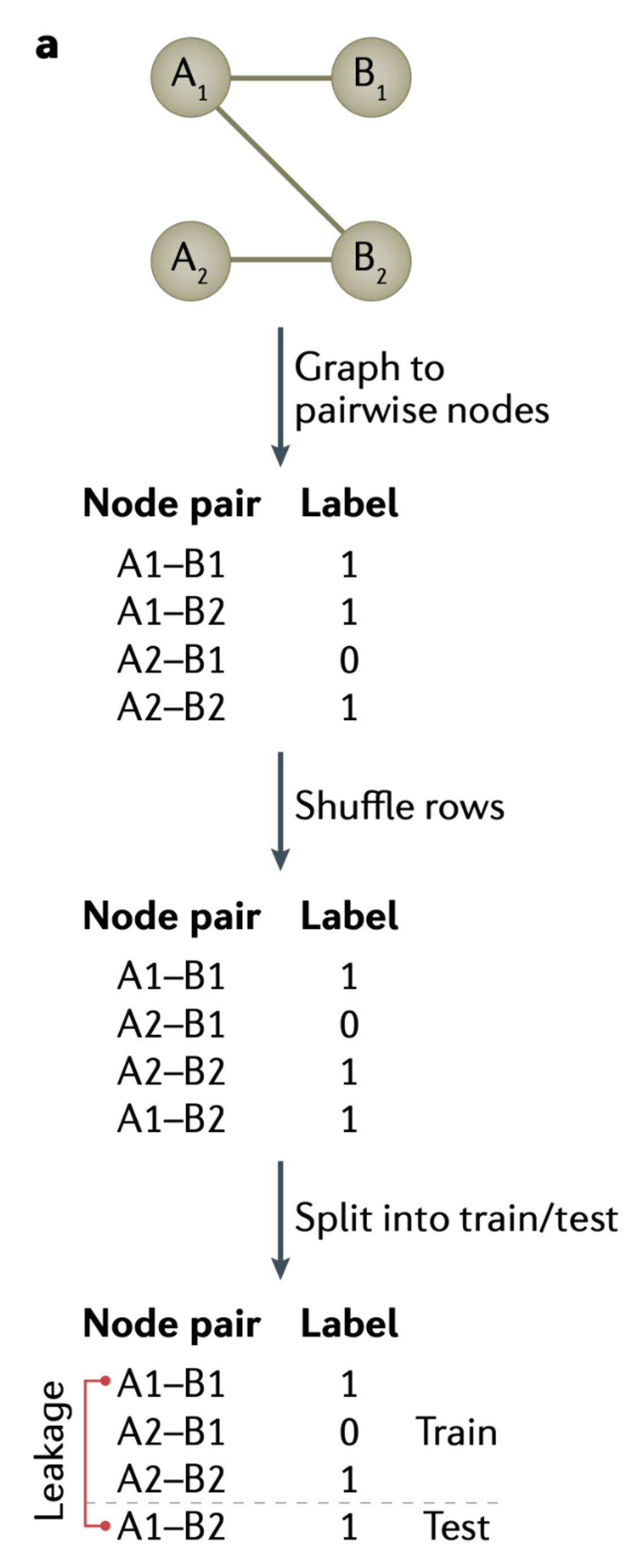
Rafi, Abdul Muntakim, Brett Kiyota, Nozomu Yachie, and Carl G de Boer. 2025. “Detecting and avoiding homology-based data leakage in genome-trained sequence models.” https://doi.org/10.1101/2025.01.22.634321.

Sokolova, Marina, and Guy Lapalme. 2009. “A systematic analysis of performance measures for classification tasks.” Information Processing and Management 45 (4): 427–37. https://doi.org/10.1016/j.ipm.2009.03.002.

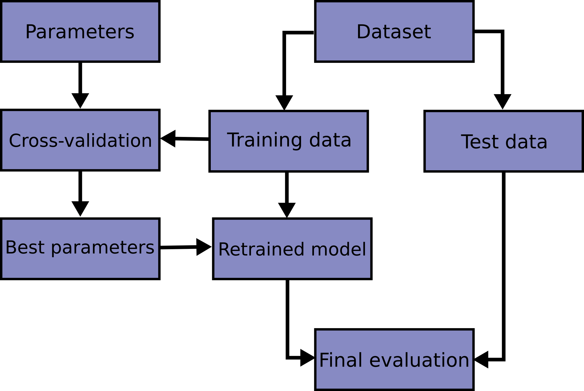
Walsh, Ian, Dmytro Fishman, Dario Garcia-Gasulla, Tiina Titma, Gianluca Pollastri, ELIXIR Machine Learning Focus Group, Emidio Capriotti, et al. 2021. “DOME: recommendations for supervised machine learning validation in biology.” Nature Methods 18 (10): 1122–27. https://doi.org/10.1038/s41592-021-01205-4.

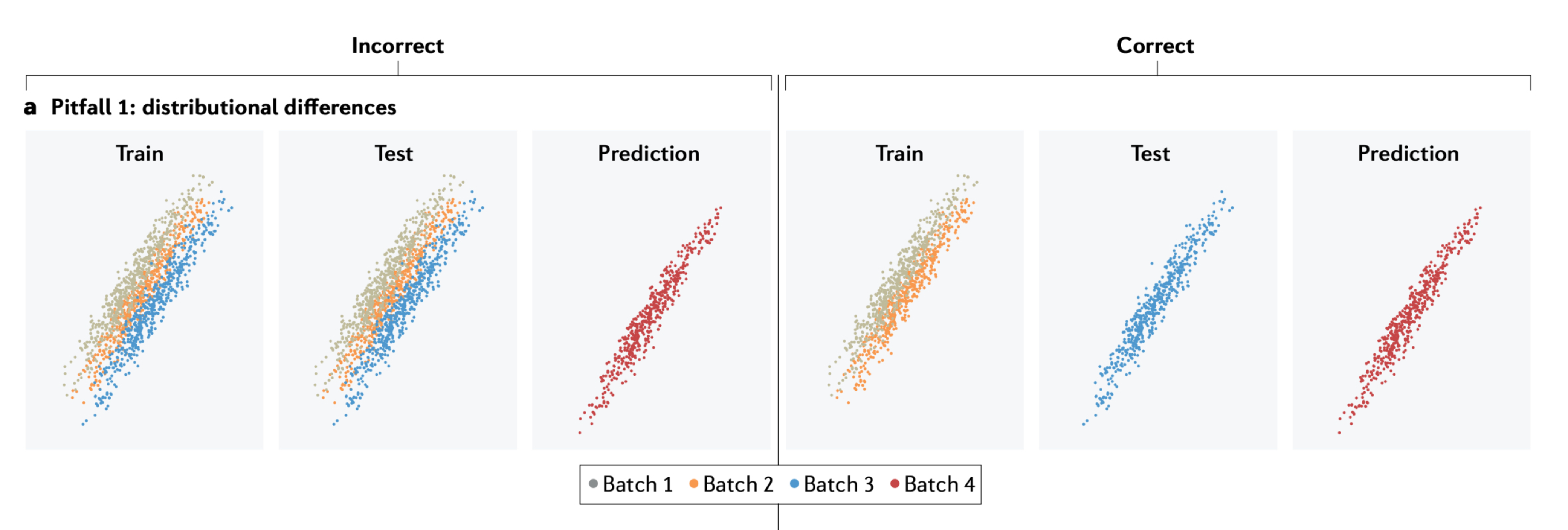
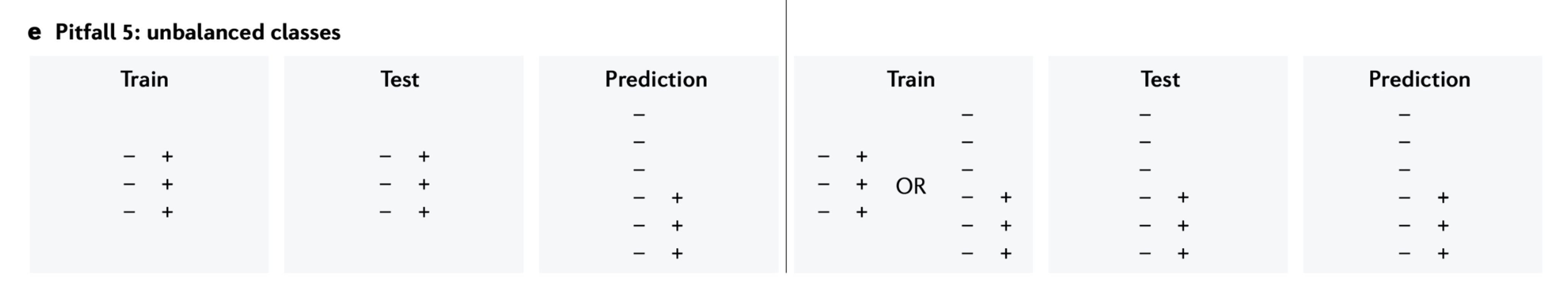
Whalen, Sean, Jacob Schreiber, William S. Noble, and Katherine S. Pollard. 2022. “Navigating the pitfalls of applying machine learning in genomics.” Nature Reviews Genetics 23 (3): 169–81. https://doi.org/10.1038/s41576-021-00434-9.

Marcel Turcotte

Marcel.Turcotte@uOttawa.ca

School of Electrical Engineering and Computer Science (EECS)

University of Ottawa