Bias-Variance Tradeoff, Model Fitting

CSI 5180 - Machine Learning for Bioinformatics

Marcel Turcotte

Version: Mar 3, 2025 09:29

Preamble

Quote of the Day (1/2)

Attribution: xkcd

Quote of the Day (2/2)

Callaway (2025)

Summary

In this lecture, we explore how model complexity influences bias, variance, and generalization by examining underfitting and overfitting through learning curves across various models, including linear, polynomial, tree-based, KNN, and deep networks.

Learning Outcomes

• Grasp how model complexity affects bias, variance, and generalization.
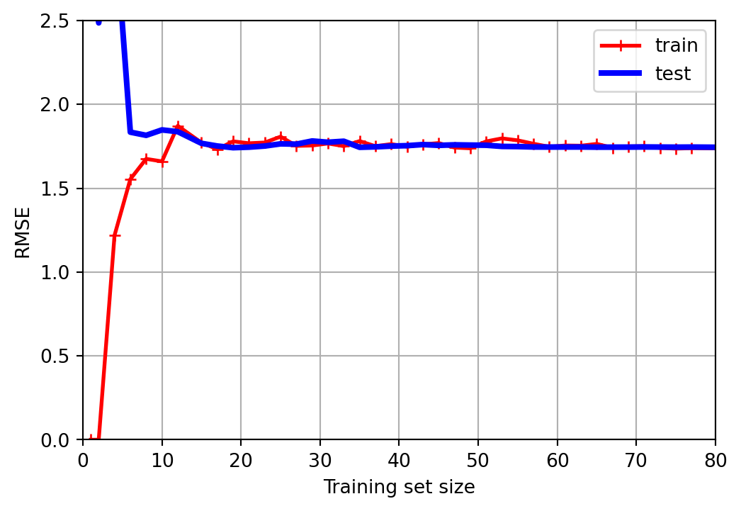
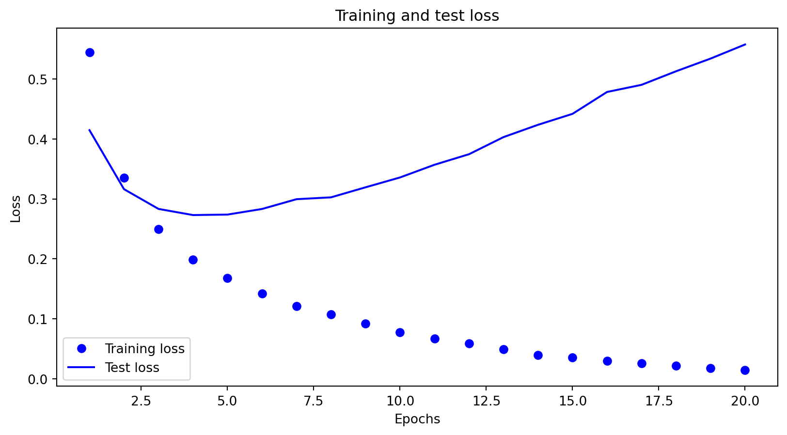
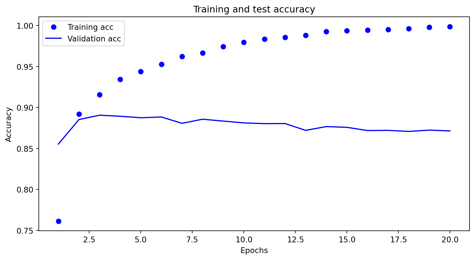
• Analyze learning curves to diagnose underfitting and overfitting.

Model Complexity

Rationale

Optimizing model performance critically depends on the careful selection and tuning of hyperparameters.

These hyperparameters play a pivotal role in regulating the complexity of machine learning models.

Definition

Model complexity in refers to the capacity of a model to capture intricate patterns in the data.

It is determined by the number of parameters or the structure of the model.

Exploration

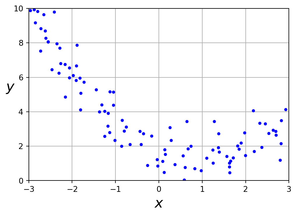
import numpy as np

np.random.seed(42)

X = 6 * np.random.rand(100, 1) - 3
y = 0.5 * X ** 2 - X + 2 + np.random.randn(100, 1)

import matplotlib as mpl
import matplotlib.pyplot as plt

plt.figure(figsize=(6,4))

plt.plot(X, y, "b.")
plt.xlabel("$x$", fontsize=18)
plt.ylabel("$y$", rotation=0, fontsize=18)
plt.axis([-3, 3, 0, 10])
plt.grid(True)
plt.show()

In machine learning experiments, specifying the seed of the random number generator is crucial for ensuring reproducibility. By setting a fixed seed, programmers can guarantee that the same sequence of random numbers will be generated each time the experiment is run. This consistency is vital for several reasons:

1. Reproducibility: It allows other programmers to replicate the experiment with the exact same conditions, facilitating verification and validation of results.
2. Comparative Analysis: It enables consistent comparison between different models or algorithms under the same initial conditions, ensuring that observed differences are due to the models themselves rather than variations in the random initialization.
3. Debugging: It aids in debugging by providing a stable environment where issues can be consistently reproduced and investigated.

Attribution: Géron (2022), Chapter 4

Linear Regression

from sklearn.linear_model import LinearRegression

lin_reg = LinearRegression()
lin_reg.fit(X, y)

X_new = np.array([[-3], [3]])
y_pred = lin_reg.predict(X_new)

plt.figure(figsize=(6,4))

plt.plot(X, y, "b.")
plt.plot(X_new, y_pred, "r-")
plt.xlabel("$x$", fontsize=18)
plt.ylabel("$y$", rotation=0, fontsize=18)
plt.axis([-3, 3, 0, 10])
plt.show()

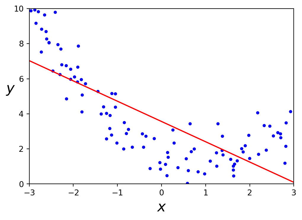
A linear model inadequately represents this dataset.

Adjusting the slope invariably leads to a scenario where residuals (errors) are minimized for certain data points while remaining significant for others.

Definition

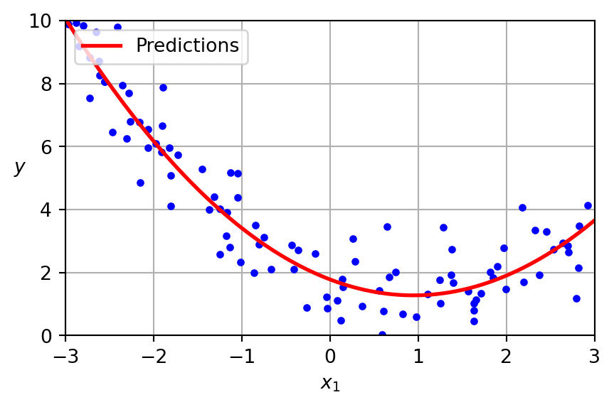
Feature engineering is the process of creating, transforming, and selecting variables (attributes) from raw data to improve the performance of machine learning models.

Here, our focus is on creating new attributes from raw data.

Machine Learning Engineering

• Machine Learning Engineering by Andriy Burkov (A. Burkov 2020).
• Covers data collection, storage, preprocessing, feature engineering, model testing and debugging, deployment, retirement, and maintenance.
• From the author of The Hundred-Page Machine Learning Book (Andriy Burkov 2019).
• Available under a “read first, buy later” model.

PolynomialFeatures

from sklearn.preprocessing import PolynomialFeatures

poly_features = PolynomialFeatures(degree=2, include_bias=False)
X_poly = poly_features.fit_transform(X)

X[0]

array([-0.75275929])

X_poly[0]

array([-0.75275929,  0.56664654])

sklearn.preprocessing.PolynomialFeatures

Generate a new feature matrix consisting of all polynomial combinations of the features with degree less than or equal to the specified degree. For example, if an input sample is two dimensional and of the form \([a, b]\), the degree-2 polynomial features are \([1, a, b, a^2, ab, b^2]\).

PolynomialFeatures

Given two features \(a\) and \(b\), PolynomialFeatures with degree=3 would add \(a^2\), \(a^3\), \(b^2\), \(b^3\), as well as, \(ab\), \(a^2b\), \(ab^2\)!

Warning

PolynomialFeatures(degree=d) adds \(\frac{(D+d)!}{d!D!}\) features, where \(D\) is the original number of features.

Additionally, you have the option to engineer new features of your own.

Polynomial Regression

lin_reg = LinearRegression()
lin_reg = lin_reg.fit(X_poly, y)

X_new = np.linspace(-3, 3, 100).reshape(100, 1)
X_new_poly = poly_features.transform(X_new)
y_new = lin_reg.predict(X_new_poly)

plt.figure(figsize=(5, 3))
plt.plot(X, y, "b.")
plt.plot(X_new, y_new, "r-", linewidth=2, label="Predictions")
plt.xlabel("$x_1$")
plt.ylabel("$y$", rotation=0)
plt.legend(loc="upper left")
plt.axis([-3, 3, 0, 10])
plt.grid()
plt.show()

LinearRegression on PolynomialFeatures

lin_reg = LinearRegression()
lin_reg.fit(X_poly, y)

Polynomial Regression

The data was generated according to the following equation, with the inclusion of Gaussian noise.

\[ y = 0.5 x^2 - 1.0 x + 2.0 \]

Presented below is the learned model.

\[ \hat{y} = 0.56 x^2 + (-1.06) x + 1.78 \]

lin_reg.coef_, lin_reg.intercept_

(array([[-1.06633107,  0.56456263]]), array([1.78134581]))

Given the noise present in our dataset, akin to what we would expect with real-world data, this model demonstrates a good fit.

Model Complexity

from sklearn.preprocessing import StandardScaler
from sklearn.pipeline import make_pipeline

plt.figure(figsize=(5, 3))

for style, width, degree in (("r-+", 2, 1), ("b--", 2, 2), ("g-", 1, 300)):
    polybig_features = PolynomialFeatures(degree=degree, include_bias=False)
    std_scaler = StandardScaler()
    lin_reg = LinearRegression()
    polynomial_regression = make_pipeline(polybig_features, std_scaler, lin_reg)
    polynomial_regression.fit(X, y)
    y_newbig = polynomial_regression.predict(X_new)
    label = f"{degree} degree{'s' if degree > 1 else ''}"
    plt.plot(X_new, y_newbig, style, label=label, linewidth=width)

plt.plot(X, y, "b.", linewidth=3)
plt.legend(loc="upper left")
plt.xlabel("$x_1$")
plt.ylabel("$y$", rotation=0)
plt.axis([-3, 3, 0, 10])
plt.grid()
plt.show()

A low loss value on the training set does not necessarily indicate a “better” model.

In this example, the linear regression model has high mean squared error (loss) on the training set (red line). This suggests that the model makes numerous errors even on the training data.

Conversely, the polynomial model with degree=300 exhibits a low mean squared error (loss) on the training set (green line), implying that it makes few errors on the training data.

However, the degree=300 polynomial model is likely to perform poorly on future predictions. The green curve extends beyond the boundaries of the image on the y-axis. For instance, for input values in the range of 2 to 3, the model predicts values exceeding 10 (as well as negative values), whereas the expected values should lie within the range of 2 to 4.

This illustrative example may seem simplistic since the data is generated from a quadratic equation and involves only a single attribute, making visualization straightforward. However, it serves to highlight a key point relevant to more complex models, such as deep neural networks. As the number of parameters increases, the model’s capacity to fit the training data also increases, which can lead to overfitting if not properly managed.

Attribution: 04_training_linear_models.ipynb

Under- and Over- Fitting

• Underfitting:
  • Your model is too simple (here, linear).
  • Uninformative features.
  • Poor performance on both training and test data.
• Overfitting:
  • Your model is too complex (tall decision tree, deep and wide neural networks, etc.).
  • Too many features given the number of examples available.
  • Excellent performance on the training set, but poor performance on the test set.

In the case of underfitting, adding more data to the training set will not help.

In the case of overfitting, adding more data would bring the train and test set learning curves closer.

Learning Curves

• One way to assess our models is to visualize the learning curves:
  • A learning curve shows the performance of our model, here using RMSE, on both the training set and the test set.
  • Multiple measurements are obtained by repeatedly training the model on larger and larger subsets of the data.

See: sklearn.model_selection.learning_curve.

Learning Curve – Underfitting

from sklearn.model_selection import learning_curve

train_sizes, train_scores, valid_scores = learning_curve(
    LinearRegression(), X, y, train_sizes=np.linspace(0.01, 1.0, 40), cv=5,
    scoring="neg_root_mean_squared_error")

train_errors = -train_scores.mean(axis=1)
valid_errors = -valid_scores.mean(axis=1)

plt.figure(figsize=(6, 4))  # extra code – not needed, just formatting
plt.plot(train_sizes, train_errors, "r-+", linewidth=2, label="train")
plt.plot(train_sizes, valid_errors, "b-", linewidth=3, label="test")

# extra code – beautifies
plt.xlabel("Training set size")
plt.ylabel("RMSE")
plt.grid()
plt.legend(loc="upper right")
plt.axis([0, 80, 0, 2.5])
plt.show()

• Polynomial with degree=1.

• Poor performance on both training and test data.

This graph illustrates the learning curve for a linear regression model applied to data generated from a quadratic equation, which serves as our ongoing example.

The horizontal axis represents the size of the training set. Initially, the linear regression model is trained on a very small dataset, consisting of just one or a few examples, and the Root Mean Square Error (RMSE) is plotted for both the training and test sets. The size of the training set is then incrementally increased, a new model is trained, and the performance is recorded. This procedure continues until the entire dataset is utilized.

Key observations from the graph include:

• With only one or two examples, the model perfectly fits the training set, resulting in low RMSE for the training data.

• As the size of the training set increases, the model struggles to fit the training data due to the quadratic nature of the data generation process. Consequently, the RMSE for the training set rises and stabilizes at a higher level.

• For small training sets, the model performs poorly on the test set due to inadequate generalization, resulting in high RMSE.

• As the training set size grows, the test set performance improves, indicated by decreasing RMSE, until it reaches a point where further increases in training set size do not yield significant improvements.

These learning curves are indicative of a model that is underfitting. Both the training and test set RMSE curves plateau at relatively high values and remain close to each other, as noted by Géron (2022).

Source code: 04_training_linear_models.ipynb.

Learning Curve – Overfitting

from sklearn.pipeline import make_pipeline

polynomial_regression = make_pipeline(
    PolynomialFeatures(degree=14, include_bias=False),
    LinearRegression())

train_sizes, train_scores, valid_scores = learning_curve(
    polynomial_regression, X, y, train_sizes=np.linspace(0.01, 1.0, 40), cv=5,
    scoring="neg_root_mean_squared_error")
# extra code – generates and saves Figure 4–16

train_errors = -train_scores.mean(axis=1)
valid_errors = -valid_scores.mean(axis=1)

plt.figure(figsize=(6, 4))
plt.plot(train_sizes, train_errors, "r-+", linewidth=2, label="train")
plt.plot(train_sizes, valid_errors, "b-", linewidth=3, label="test")
plt.legend(loc="upper right")
plt.xlabel("Training set size")
plt.ylabel("RMSE")
plt.grid()
plt.axis([0, 80, 0, 2.5])
plt.show()

• Polynomial with degree=14.

• Excellent performance on the training set, but poor performance on the test set.

• For a training set of up to 14 data points, the polynomial fits the training data perfectly, resulting in an RMSE of zero.

• The error on the training data in this instance is significantly lower.

• A notable gap between the two curves indicates that the model performs substantially better on the training data compared to the test data.

Overfitting - Deep Net - Loss

Neural networks will be covered in detail later in our course. The graph presented here illustrates the variation in the loss function as a deep learning model undergoes training.

This example utilizes the IMDB movie review sentiment classification dataset available in Keras. The dataset comprises 25,000 movie reviews from IMDB, each labeled with a sentiment (positive or negative).

The model consists of three dense layers with sizes 16, 16, and 1, respectively. It includes a total of 160,305 trainable parameters.

The network is trained using mini-batch stochastic gradient descent with a batch size of 512. The horizontal axis represents the number of epochs, where each epoch indicates that the model has seen the entire training set once. During each epoch, the stochastic gradient descent algorithm updates the model parameters iteratively using mini-batches of 512 examples.

I selected this example to illustrate that a neural network with with sufficient capacity (number of parameters) can minimize training errors almost to zero, as reducing training error is the primary objective of optimization. However, the graph clearly demonstrates that beyond a certain point, the learned patterns become specific to the training set rather than general principles. Generalization, rather than mere memorization, is the ultimate goal of machine learning.

Overfitting occurs when a model learns the details and noise in the training data to an extent that it negatively impacts the model’s performance on new data. This can result in a decision boundary that fits the training data too tightly, capturing noise and irrelevant details rather than general patterns.

Example from Chollet (2017) Chapter 3 (chapter04_getting-started-with-neural-networks.ipynb, ipynb from 2021 edition).

Overfitting - Deep Net - Accuracy

This graph similarly illustrates the variation in accuracy for both the training and test sets as the model undergoes training.

Bias-Variance Tradeoff

Bias

• Bias refers to the error introduced by approximating a real-world problem, which may be complex, using a simplified model.

• It represents the difference between the average prediction of the model and the true outcome.

• High bias can cause an algorithm to miss important patterns, leading to underfitting.

Bias

\[ \text{Bias}(\hat{f}) = \mathbb{E}[\hat{f}(x)] - f(x) \] where:

• \(\hat{f}(x)\) is the prediction made by the model,
• \(f(x)\) is the true function,
• \(\mathbb{E}[\hat{f}(x)]\) is the expected prediction over different datasets.

Variance

• Variance measures the model’s sensitivity to fluctuations in the training data.

• High variance indicates that the model is capturing noise as if it were a true pattern, leading to overfitting.

• It reflects how much the predictions of the model would vary if different training data were used.

Variance

\[ \text{Variance}(\hat{f}) = \mathbb{E}[(\hat{f}(x) - \mathbb{E}[\hat{f}(x)])^2] \]

where:

• \(\hat{f}(x)\) is the prediction made by the model,
• \(\mathbb{E}[\hat{f}(x)]\) is the expected prediction over different datasets.

Remarks

• Statistical learning makes assumptions about the model, data distribution, and noise to analytically derive expected values.

• In practical applications, empirical techniques like cross-validation and bootstrapping are employed to estimate bias and variance.

Bais-Variance Tradeoff

\[ \text{Error} = \text{Bias}^2 + \text{Variance} + \text{Irreducible Error} \]

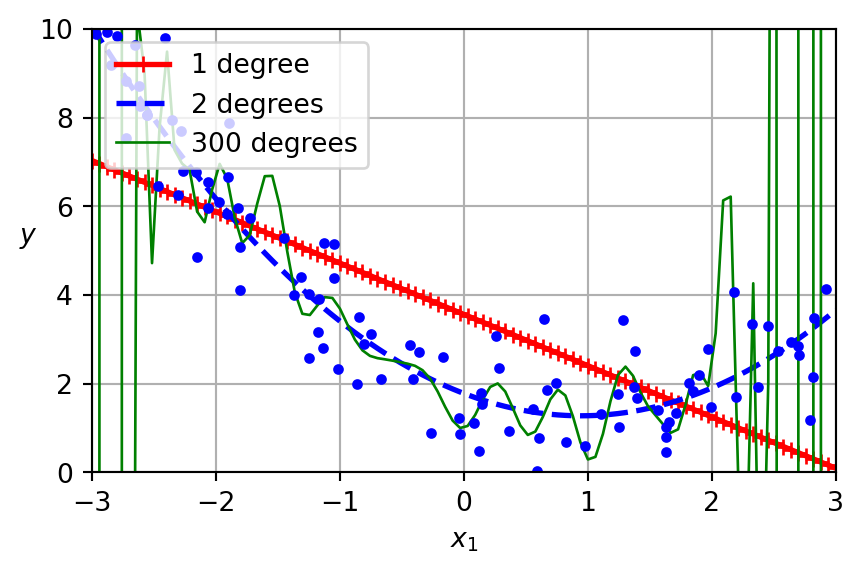
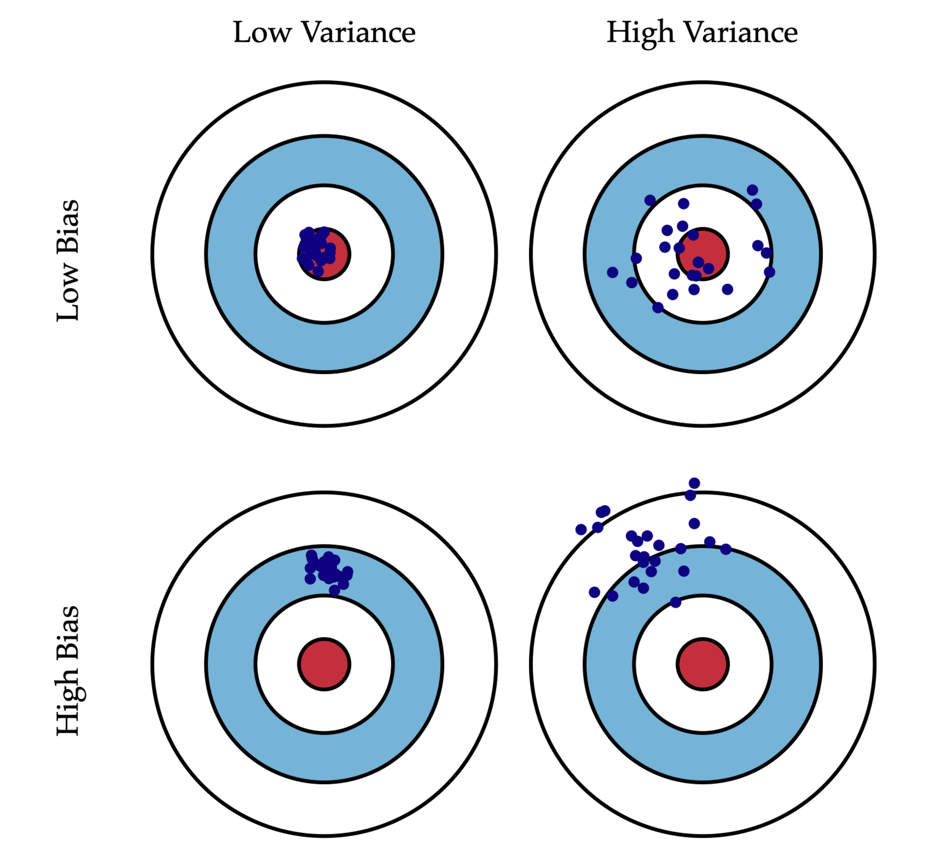
• Model selection aims to minimize bias, which arises from overly simplistic models, and variance, which results from overly complex models prone to overfitting.

• Ideally, with infinite data, both bias and variance could be reduced to zero.

• However, in practice, data is typically noisy, and some irreducible error persists due to unaccounted factors beyond the model’s scope.

Strive for a model complexity that captures essential patterns without tipping into overfitting.

Bais-Variance Tradeoff

Attribution: Bigbossfarin, CC0, via Wikimedia Commons

Bais-Variance Tradeoff

Attribution: Understanding the Bias-Variance Tradeoff by Scott Fortmann-Roe, June 2012.

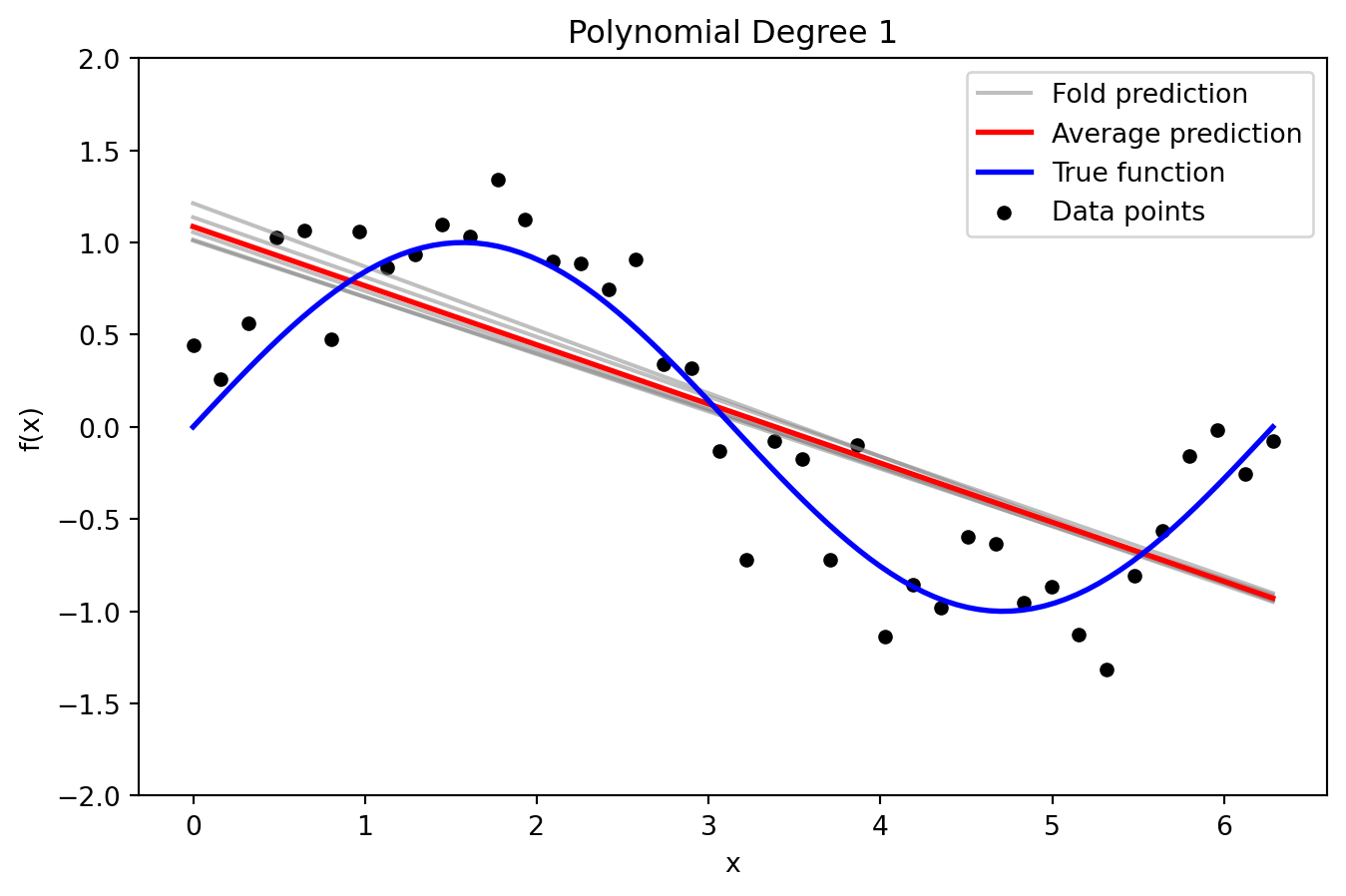
High Bias, Low Variance

from sklearn.model_selection import KFold
from sklearn.metrics import mean_squared_error

def true_function(x):
    return np.sin(x)

def plot_fold_predictions(degree, X, y, X_grid, y_true_grid, n_splits=5, random_state=42):
    """
    For a given polynomial degree, perform KFold cross-validation,
    plot the individual fold predictions along with the average prediction 
    and the true function (with y-axis limited to [-2, 2]),
    and return predictions and errors.
    """
    kf = KFold(n_splits=n_splits, shuffle=True, random_state=random_state)
    fold_predictions = []  # To store predictions on the evaluation grid for each fold
    fold_errors = []       # To store test errors for each fold

    for train_index, test_index in kf.split(X):
        poly = PolynomialFeatures(degree=degree)
        X_train_poly = poly.fit_transform(X[train_index])
        X_test_poly = poly.transform(X[test_index])
        X_grid_poly = poly.transform(X_grid)
        
        model = LinearRegression()
        model.fit(X_train_poly, y[train_index])
        
        # Predictions on the dense grid for bias-variance analysis
        y_pred_grid = model.predict(X_grid_poly)
        fold_predictions.append(y_pred_grid)
        
        # Test error on held-out data
        y_pred_test = model.predict(X_test_poly)
        fold_errors.append(mean_squared_error(y[test_index], y_pred_test))
    
    fold_predictions = np.array(fold_predictions)
    avg_prediction = np.mean(fold_predictions, axis=0)
    
    # Plot individual fold predictions with y-axis limited to [-2, 2]
    plt.figure(figsize=(8, 5))
    for i in range(n_splits):
        plt.plot(X_grid, fold_predictions[i], color='gray', alpha=0.5, 
                 label='Fold prediction' if i == 0 else "")
    plt.plot(X_grid, avg_prediction, color='red', linewidth=2, label='Average prediction')
    plt.plot(X_grid, y_true_grid, color='blue', linewidth=2, label='True function')
    plt.scatter(X, y, color='black', s=20, label='Data points')
    plt.ylim(-2, 2)
    plt.title(f'Polynomial Degree {degree}')
    plt.xlabel('x')
    plt.ylabel('f(x)')
    plt.legend()
    plt.show()
    
    return fold_predictions, avg_prediction, fold_errors

# --- Data Generation with Increased Noise and Reduced Sample Size ---
np.random.seed(0)
n_samples = 40  # Reduced sample size increases model sensitivity to training data
X = np.linspace(0, 2 * np.pi, n_samples).reshape(-1, 1)
noise_std = 0.25  # Increased noise level amplifies prediction variability
y = true_function(X).ravel() + np.random.normal(0, noise_std, size=n_samples)

# Create a dense evaluation grid and compute the true function values
X_grid = np.linspace(0, 2 * np.pi, 100).reshape(-1, 1)
y_true_grid = true_function(X_grid).ravel()

# --- Plot Individual Fold Predictions for Selected Degrees ---
_ = plot_fold_predictions(1, X, y, X_grid, y_true_grid, n_splits=5)

• High Bias: The model lacks complexity and, consequently, fails to capture the underlying patterns in the data, resulting in a high average error.

• Low Variance: The model exhibits insensitivity to variations in the dataset, which manifests as low variance.

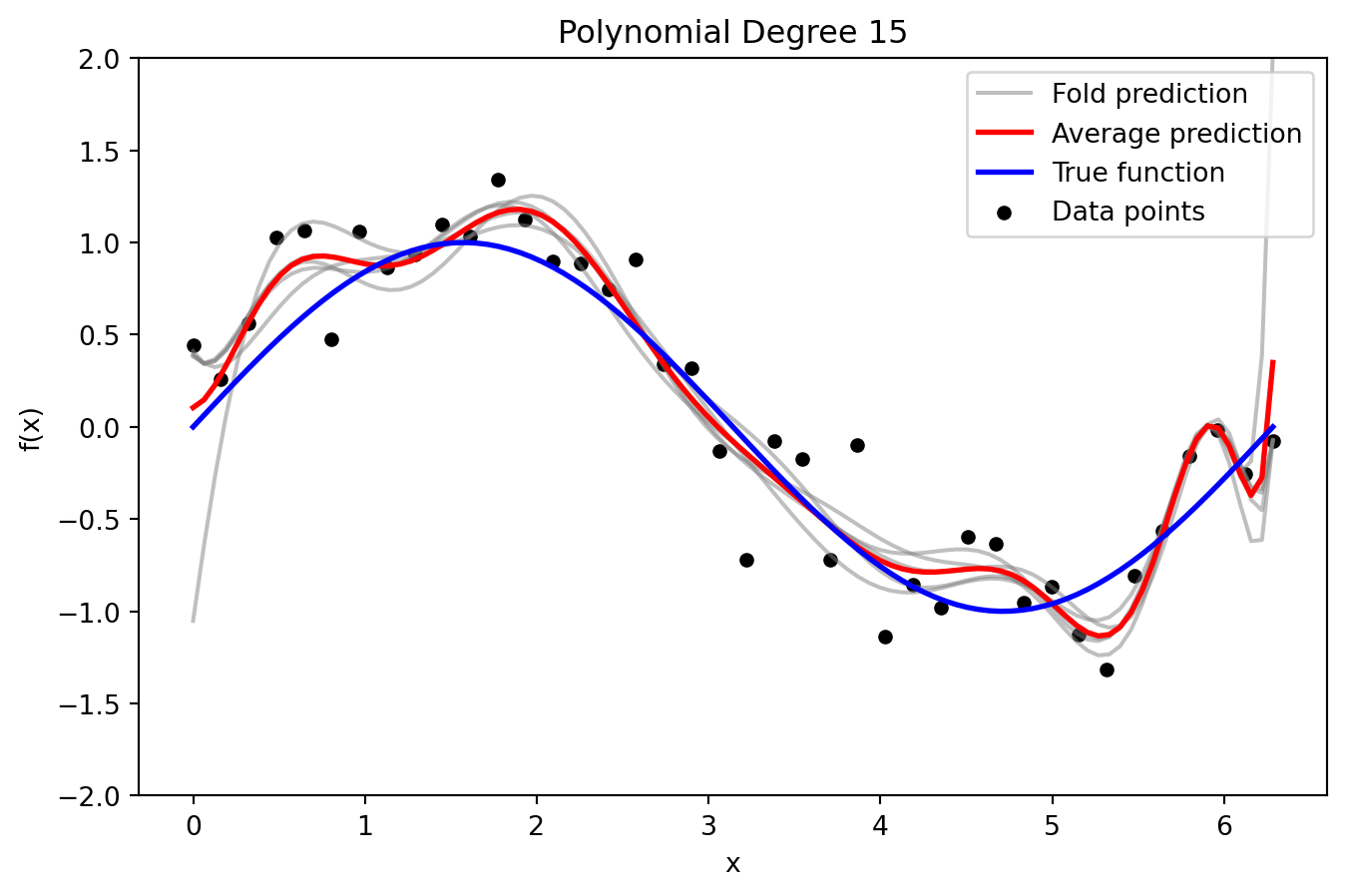
Low Bias, High Variance

_ = plot_fold_predictions(15, X, y, X_grid, y_true_grid, n_splits=5)

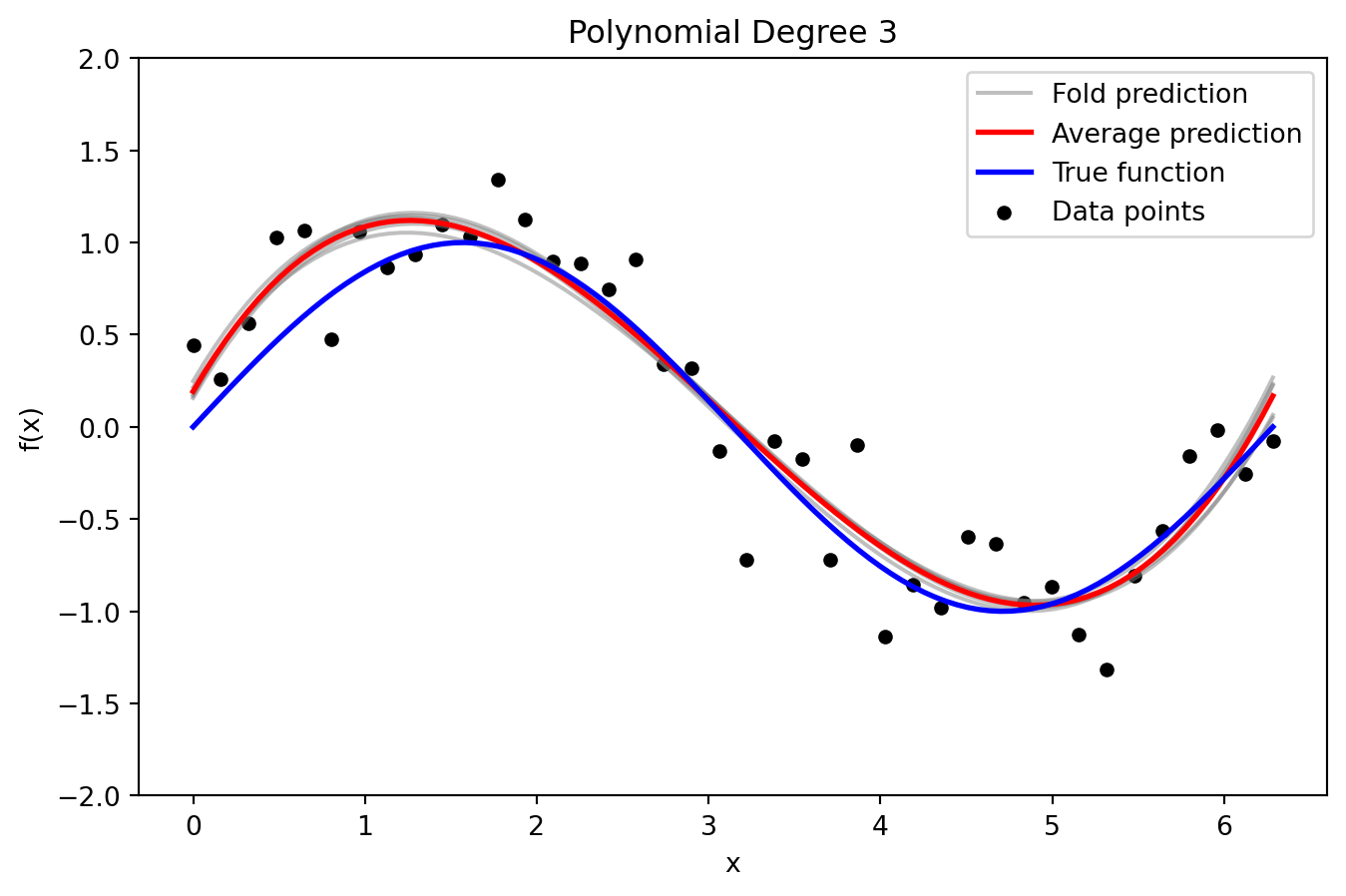
Just Right

_ = plot_fold_predictions(3, X, y, X_grid, y_true_grid, n_splits=5)

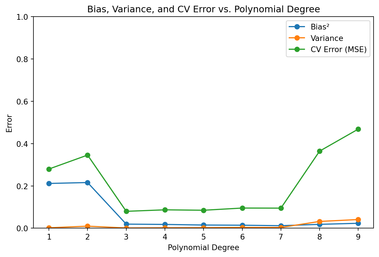
Bias, Variance, and CV Error

# --- Compute Bias², Variance, and CV Error Across Degrees 1 to 10 ---
degrees = range(1, 10)
bias_list = []
variance_list = []
cv_error_list = []

for degree in degrees:
    kf = KFold(n_splits=5, shuffle=True, random_state=42)
    fold_predictions = []
    fold_errors = []
    
    for train_index, test_index in kf.split(X):
        poly = PolynomialFeatures(degree=degree)
        X_train_poly = poly.fit_transform(X[train_index])
        X_test_poly = poly.transform(X[test_index])
        X_grid_poly = poly.transform(X_grid)
        
        model = LinearRegression()
        model.fit(X_train_poly, y[train_index])
        
        y_pred_grid = model.predict(X_grid_poly)
        fold_predictions.append(y_pred_grid)
        
        y_pred_test = model.predict(X_test_poly)
        fold_errors.append(mean_squared_error(y[test_index], y_pred_test))
    
    fold_predictions = np.array(fold_predictions)
    mean_prediction = np.mean(fold_predictions, axis=0)
    
    # Bias²: Average squared difference between the average prediction and the true function
    bias_sq = np.mean((mean_prediction - y_true_grid)**2)
    # Variance: Average variance of the predictions across the evaluation grid
    variance = np.mean(np.var(fold_predictions, axis=0))
    # CV Error: Mean of the MSE on held-out test sets
    cv_error = np.mean(fold_errors)
    
    bias_list.append(bias_sq)
    variance_list.append(variance)
    cv_error_list.append(cv_error)

# --- Plot Bias², Variance, and CV Error vs. Polynomial Degree ---
plt.figure(figsize=(8, 5))
plt.plot(degrees, bias_list, marker='o', label='Bias²')
plt.plot(degrees, variance_list, marker='o', label='Variance')
plt.plot(degrees, cv_error_list, marker='o', label='CV Error (MSE)')
plt.title('Bias, Variance, and CV Error vs. Polynomial Degree')
plt.xlabel('Polynomial Degree')
plt.ylabel('Error')
plt.ylim(0, 1)
plt.legend()
plt.show()

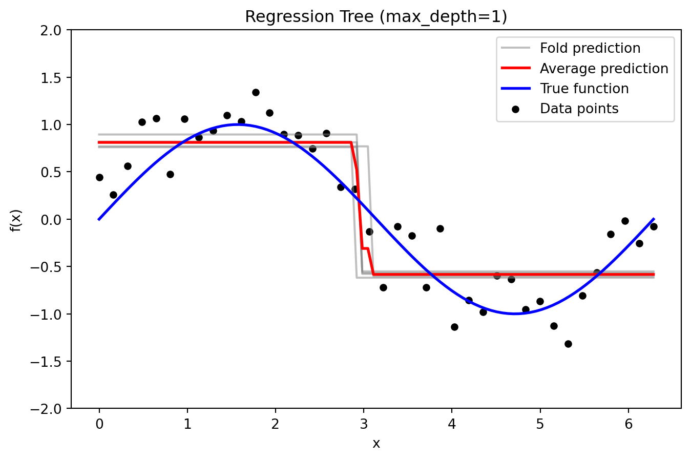
Regression Tree

from sklearn.tree import DecisionTreeRegressor

def plot_tree_fold_predictions(max_depth, X, y, X_grid, y_true_grid, n_splits=5, random_state=42):
    """
    For a given tree max_depth, perform KFold cross-validation with a DecisionTreeRegressor,
    plot the individual fold predictions along with the average prediction and the true function.
    The y-axis is limited to [-2, 2] for clarity.
    """
    kf = KFold(n_splits=n_splits, shuffle=True, random_state=random_state)
    fold_predictions = []  # Store predictions on the evaluation grid for each fold
    fold_errors = []       # Store test errors for each fold

    for train_index, test_index in kf.split(X):
        X_train = X[train_index]
        X_test = X[test_index]
        
        model = DecisionTreeRegressor(max_depth=max_depth, random_state=random_state)
        model.fit(X_train, y[train_index])
        
        # Prediction on a dense evaluation grid
        y_pred_grid = model.predict(X_grid)
        fold_predictions.append(y_pred_grid)
        
        # Test error on held-out data
        y_pred_test = model.predict(X_test)
        fold_errors.append(mean_squared_error(y[test_index], y_pred_test))
    
    fold_predictions = np.array(fold_predictions)
    avg_prediction = np.mean(fold_predictions, axis=0)
    
    plt.figure(figsize=(8, 5))
    for i in range(n_splits):
        plt.plot(X_grid, fold_predictions[i], color='gray', alpha=0.5,
                 label='Fold prediction' if i == 0 else "")
    plt.plot(X_grid, avg_prediction, color='red', linewidth=2, label='Average prediction')
    plt.plot(X_grid, y_true_grid, color='blue', linewidth=2, label='True function')
    plt.scatter(X, y, color='black', s=20, label='Data points')
    plt.ylim(-2, 2)
    plt.title(f'Regression Tree (max_depth={max_depth})')
    plt.xlabel('x')
    plt.ylabel('f(x)')
    plt.legend()
    plt.show()
    
    return fold_predictions, avg_prediction, fold_errors

# --- Plot Individual Fold Predictions for Selected Tree Depths ---
_ = plot_tree_fold_predictions(1, X, y, X_grid, y_true_grid, n_splits=5)

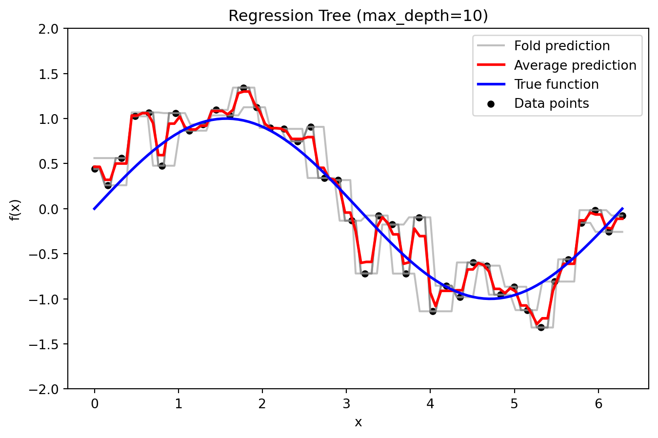
Regression Tree

_ = plot_tree_fold_predictions(10, X, y, X_grid, y_true_grid, n_splits=5)

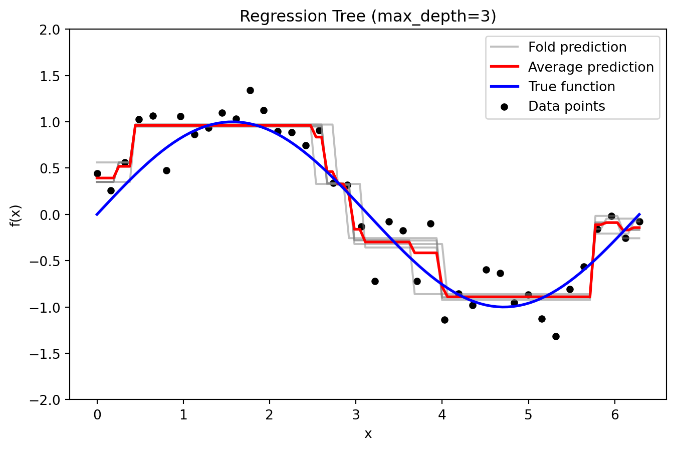
Regression Tree

_ = plot_tree_fold_predictions(3, X, y, X_grid, y_true_grid, n_splits=5)

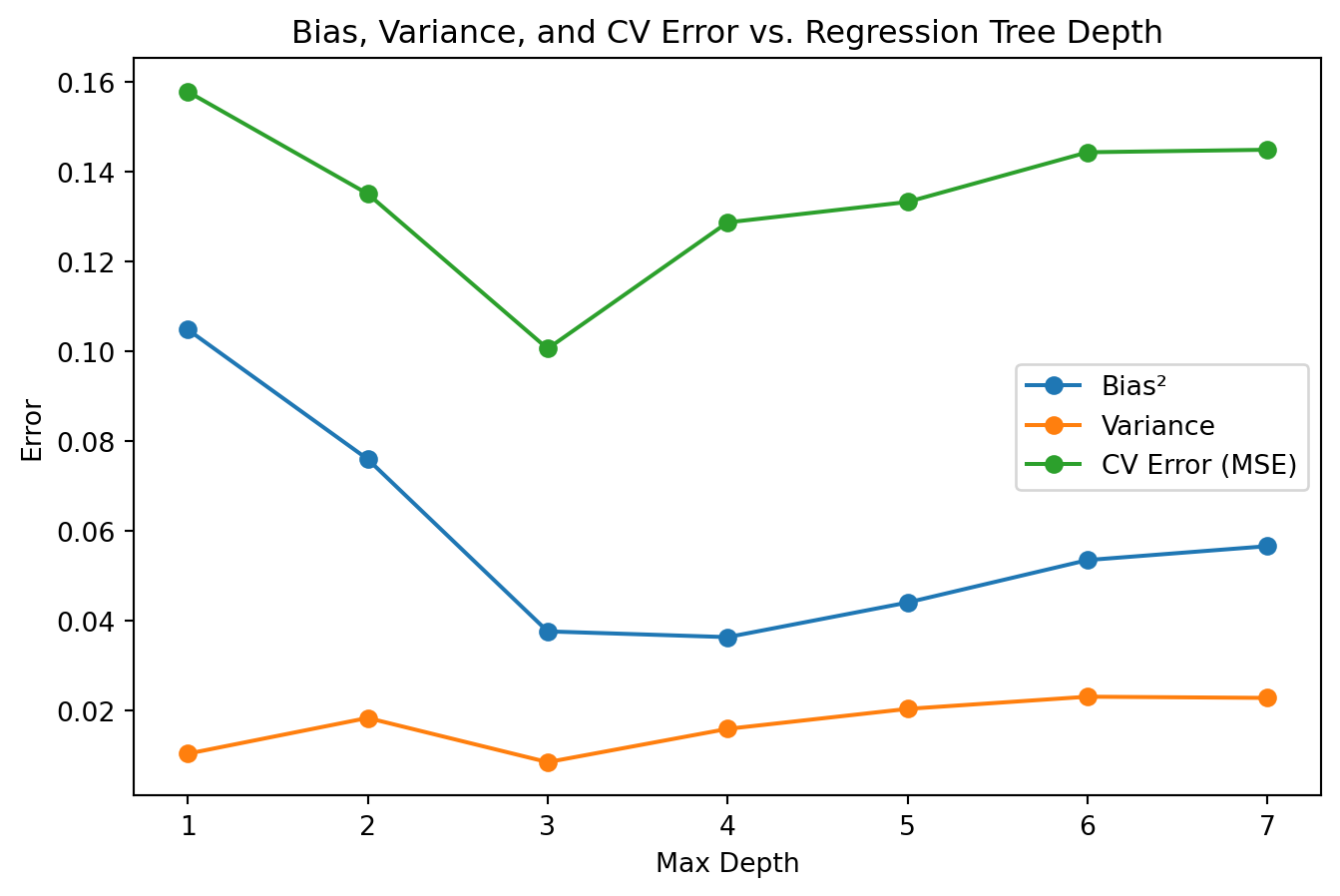
Bias, Variance, and CV Error

# --- Compute Bias², Variance, and CV Error vs. Tree Depth ---
max_depths = range(1, 8)
bias_list = []
variance_list = []
cv_error_list = []

for depth in max_depths:
    kf = KFold(n_splits=5, shuffle=True, random_state=42)
    fold_predictions = []
    fold_errors = []
    
    for train_index, test_index in kf.split(X):
        X_train = X[train_index]
        X_test = X[test_index]
        
        model = DecisionTreeRegressor(max_depth=depth, random_state=42)
        model.fit(X_train, y[train_index])
        
        y_pred_grid = model.predict(X_grid)
        fold_predictions.append(y_pred_grid)
        
        y_pred_test = model.predict(X_test)
        fold_errors.append(mean_squared_error(y[test_index], y_pred_test))
    
    fold_predictions = np.array(fold_predictions)
    mean_prediction = np.mean(fold_predictions, axis=0)
    
    # Bias²: Mean squared difference between the average prediction and the true function
    bias_sq = np.mean((mean_prediction - y_true_grid)**2)
    # Variance: Average variance of predictions across the evaluation grid
    variance = np.mean(np.var(fold_predictions, axis=0))
    # CV Error: Average test error over folds
    cv_error = np.mean(fold_errors)
    
    bias_list.append(bias_sq)
    variance_list.append(variance)
    cv_error_list.append(cv_error)

plt.figure(figsize=(8, 5))
plt.plot(max_depths, bias_list, marker='o', label='Bias²')
plt.plot(max_depths, variance_list, marker='o', label='Variance')
plt.plot(max_depths, cv_error_list, marker='o', label='CV Error (MSE)')
plt.title('Bias, Variance, and CV Error vs. Regression Tree Depth')
plt.xlabel('Max Depth')
plt.ylabel('Error')
# plt.ylim(0, 1)
plt.legend()
plt.show()

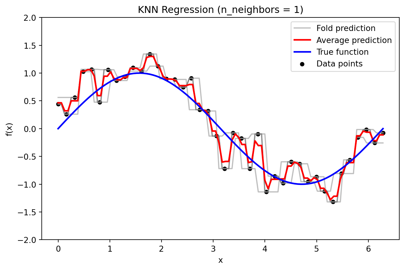
KNN Regression

from sklearn.neighbors import KNeighborsRegressor

def plot_knn_fold_predictions(n_neighbors, X, y, X_grid, y_true_grid, n_splits=5, random_state=42):
    """
    For a given number of neighbors, perform KFold cross-validation using KNeighborsRegressor,
    plot the predictions from each fold along with the average prediction and the true function.
    The y-axis is limited to [-2, 2] for clarity.
    """
    kf = KFold(n_splits=n_splits, shuffle=True, random_state=random_state)
    fold_predictions = []  # Store predictions on the evaluation grid for each fold
    fold_errors = []       # Store test errors for each fold

    for train_index, test_index in kf.split(X):
        X_train = X[train_index]
        X_test = X[test_index]
        
        model = KNeighborsRegressor(n_neighbors=n_neighbors)
        model.fit(X_train, y[train_index])
        
        # Prediction on a dense evaluation grid for bias-variance analysis
        y_pred_grid = model.predict(X_grid)
        fold_predictions.append(y_pred_grid)
        
        # Test error on held-out data
        y_pred_test = model.predict(X_test)
        fold_errors.append(mean_squared_error(y[test_index], y_pred_test))
    
    fold_predictions = np.array(fold_predictions)
    avg_prediction = np.mean(fold_predictions, axis=0)
    
    # Plot individual fold predictions
    plt.figure(figsize=(8, 5))
    for i in range(n_splits):
        plt.plot(X_grid, fold_predictions[i], color='gray', alpha=0.5,
                 label='Fold prediction' if i == 0 else "")
    plt.plot(X_grid, avg_prediction, color='red', linewidth=2, label='Average prediction')
    plt.plot(X_grid, y_true_grid, color='blue', linewidth=2, label='True function')
    plt.scatter(X, y, color='black', s=20, label='Data points')
    plt.ylim(-2, 2)
    plt.title(f'KNN Regression (n_neighbors = {n_neighbors})')
    plt.xlabel('x')
    plt.ylabel('f(x)')
    plt.legend()
    plt.show()
    
    return fold_predictions, avg_prediction, fold_errors

# --- Plot Individual Fold Predictions for Selected Values of k ---
_ = plot_knn_fold_predictions(1, X, y, X_grid, y_true_grid, n_splits=5)

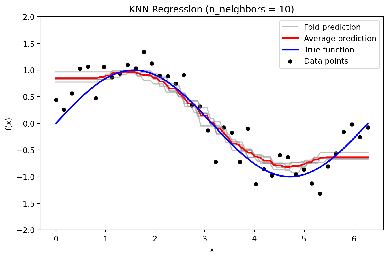
KNN Regression

_ = plot_knn_fold_predictions(10, X, y, X_grid, y_true_grid, n_splits=5)

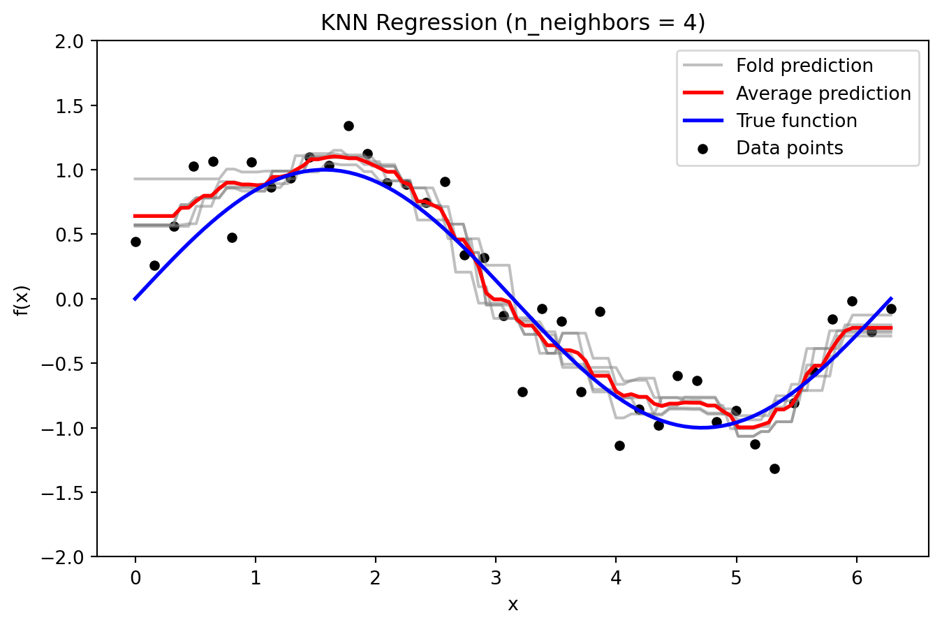
KNN Regression

_ = plot_knn_fold_predictions(4, X, y, X_grid, y_true_grid, n_splits=5)

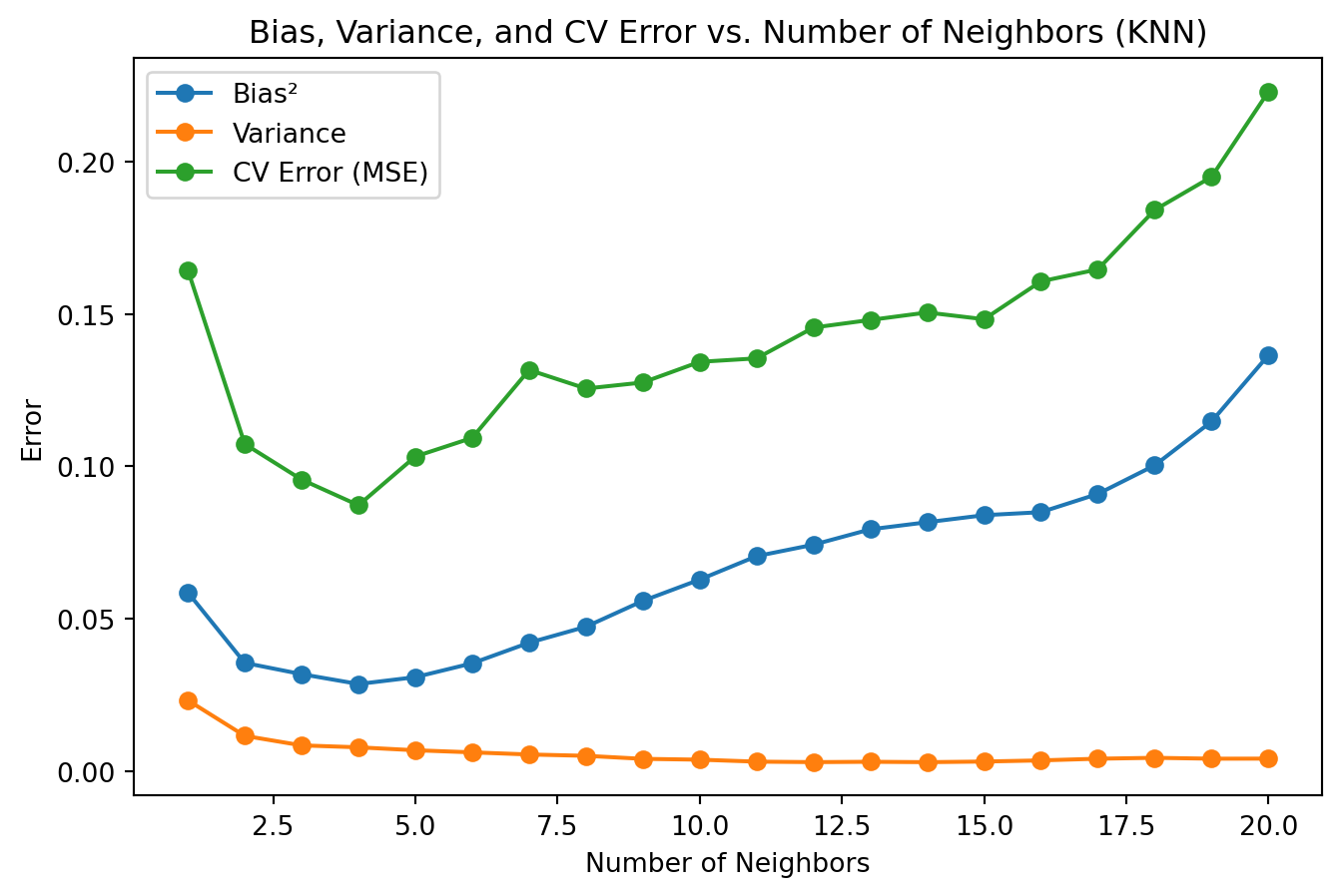
Bias, Variance, and CV Error

# --- Compute Bias², Variance, and CV Error vs. Number of Neighbors ---
neighbors_range = range(1, 21)  # Vary k from 1 to 20
bias_list = []
variance_list = []
cv_error_list = []

for k in neighbors_range:
    kf = KFold(n_splits=5, shuffle=True, random_state=42)
    fold_predictions = []
    fold_errors = []
    
    for train_index, test_index in kf.split(X):
        X_train = X[train_index]
        X_test = X[test_index]
        
        model = KNeighborsRegressor(n_neighbors=k)
        model.fit(X_train, y[train_index])
        
        y_pred_grid = model.predict(X_grid)
        fold_predictions.append(y_pred_grid)
        
        y_pred_test = model.predict(X_test)
        fold_errors.append(mean_squared_error(y[test_index], y_pred_test))
    
    fold_predictions = np.array(fold_predictions)
    mean_prediction = np.mean(fold_predictions, axis=0)
    
    # Bias²: Mean squared difference between the average prediction and the true function
    bias_sq = np.mean((mean_prediction - y_true_grid)**2)
    # Variance: Average variance of predictions across the evaluation grid
    variance = np.mean(np.var(fold_predictions, axis=0))
    # CV Error: Average MSE on the held-out test sets
    cv_error = np.mean(fold_errors)
    
    bias_list.append(bias_sq)
    variance_list.append(variance)
    cv_error_list.append(cv_error)

# --- Plot Bias², Variance, and CV Error vs. Number of Neighbors ---
plt.figure(figsize=(8, 5))
plt.plot(neighbors_range, bias_list, marker='o', label='Bias²')
plt.plot(neighbors_range, variance_list, marker='o', label='Variance')
plt.plot(neighbors_range, cv_error_list, marker='o', label='CV Error (MSE)')
plt.title('Bias, Variance, and CV Error vs. Number of Neighbors (KNN)')
plt.xlabel('Number of Neighbors')
plt.ylabel('Error')
# plt.ylim(0, 1)
plt.legend()
plt.show()

At first, this might seem counterintuitive, but it’s a direct consequence of how KNN works.

With a very low \(k\) (e.g., \(k = 1\)), the model makes predictions based on the single closest neighbor, capturing almost every detail of the training data—this yields low bias but high variance because the predictions are highly sensitive to noise.

In contrast, a higher \(k\) forces the regressor to average over many neighbors, which smooths out the predictions. This results in a simpler, less flexible model that might not capture local nuances (high bias) but is less sensitive to fluctuations in the training set (low variance).

How do you explain that Bias\(^2\) increases with the value of \(k\)?

Prologue

Summary

• Evaluated model complexity and its impact on performance.
• Illustrated underfitting, overfitting, and the bias–variance tradeoff.
• Demonstrated learning curves and cross-validation across diverse models (linear, polynomial, tree, KNN, deep nets).

Next lecture

• Machine Learning Engineering

References

Ambroise, Christophe, and Geoffrey J. McLachlan. 2002. “Selection bias in gene extraction on the basis of microarray gene-expression data.” Proceedings of the National Academy of Sciences 99 (10): 6562–66. https://doi.org/10.1073/pnas.102102699.

Burkov, A. 2020. Machine Learning Engineering. True Positive Incorporated. https://books.google.ca/books?id=HeXizQEACAAJ.

Burkov, Andriy. 2019. The Hundred-Page Machine Learning Book. Andriy Burkov.

Callaway, Ewen. 2025. “Biggest-ever AI biology model writes DNA on demand.” Nature 638 (8052): 868–69. https://doi.org/10.1038/d41586-025-00531-3.

Chollet, François. 2017. Deep Learning with Python. Manning Publications.

Géron, Aurélien. 2022. Hands-on Machine Learning with Scikit-Learn, Keras, and TensorFlow. 3rd ed. O’Reilly Media, Inc.

Libbrecht, Maxwell W, and William Stafford Noble. 2015. “Machine learning applications in genetics and genomics.” Nature Reviews Genetics 16 (6): 321–32. https://doi.org/10.1038/nrg3920.

Statnikov, Alexander, Constantin F. Aliferis, Ioannis Tsamardinos, Douglas Hardin, and Shawn Levy. 2004. “A comprehensive evaluation of multicategory classification methods for microarray gene expression cancer diagnosis.” Bioinformatics 21 (5): 631–43. https://doi.org/10.1093/bioinformatics/bti033.

Marcel Turcotte

Marcel.Turcotte@uOttawa.ca

School of Electrical Engineering and Computer Science (EECS)

University of Ottawa