Deap Learning Training

CSI 5180 - Machine Learning for Bioinformatics

Marcel Turcotte

Version: Mar 11, 2025 10:27

Preamble

Quote of the Day

AI tools are spotting errors in research papers: inside a growing movement by Elizabeth Gibney in Nature News, 2025-03-07.

Summary

This lecture provides an in‐depth introduction to deep learning training with a focus on its applications in bioinformatics. It covers the key models and repositories used in genomics—such as Kipoi, Hugging Face, and DragoNN—while explaining the fundamental components of neural networks including layers, activation functions, and the universal approximation theorem. The lecture then delves into the mechanics of training neural networks, detailing the forward pass, backpropagation, gradient descent, and techniques for overcoming challenges like vanishing and exploding gradients through proper weight initialization, dropout, and early stopping.

Learning Objectives

• Understand the core architecture and components of deep neural networks.
• Explain the role and differences among activation functions and their impact on training.
• Describe the backpropagation algorithm and its significance in updating network weights.
• Identify common challenges in training deep networks and the strategies used to overcome them.
• Recognize key genomics-specific deep learning resources and repositories.

Models for Genomics

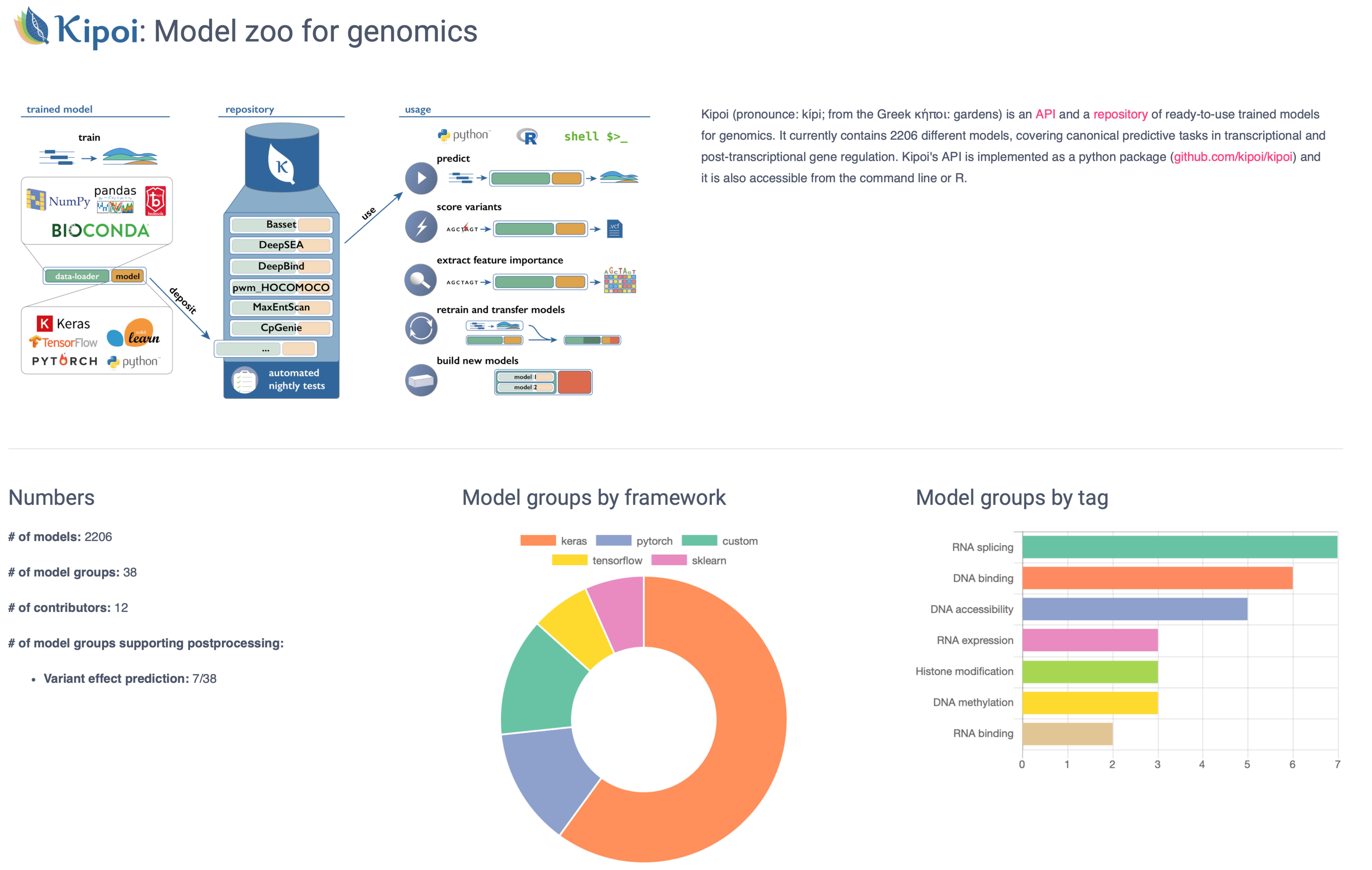
Kipoi

Kipoi is an open science initiative that provides a repository for sharing and reusing trained machine learning models in genomics. It offers over 2,000 models for tasks like predicting chromatin accessibility and transcription factor binding. Kipoi includes standardized data handling, an API for easy integration, and supports model adaptation through retraining or combination. It facilitates reproducible research by automating model installation and testing.

Avsec et al. (2019)

Kipoi (Continued)

import kipoi

model = kipoi.get_model("Basset") # load the model

model.predict_on_batch(x)

## or

model.pipeline.predict(dict(fasta_file="hg19.fa", intervals_file="intervals.bed"))

kipoi.org, example notebooks, predicting transcription factor binding sites

Hugging Face, Inc. 

• A private company develops computational tools for machine learning applications, known for its NLP-focused transformers library.
• It provides a platform for sharing machine learning models and datasets, featuring hundreds of resources related to DNA, RNA, protein, and biology.

As of March 11, 2025, Hugging Face hosts 1,493,491 models and 328,402 datasets.

Popular models available for download include DeepSeek R1 and Qwen QwQ-32B.

Hugging Face, Inc. (Continued)

• Example
  • AIDO.Protein-16B
    • AIDO.Protein-16B is a protein language model, trained on 1.2 trillion amino acids sourced from UniRef90 and ColabFoldDB.
    • Mixture of Experts Enable Efficient and Effective Protein Understanding and Design

huggingface.co

DragoNN

• Toolkit to learn how to model and interpret regulatory sequence data using deep learning.
  • Exploring convolutional neural network (CNN) architectures for a homotypic motif density simulation.
  • CNN hyperparameter tuning via grid search.
  • Interpreting features induced by CNN’s across multiple types of motif grammars.
  • Interpreting predictive sequence features in TF binding events within the GM12878 cell line.
  • Functional variant characterization for non-coding SNPs within the SPI1 motif.

The software is maintained by Johnny Israeli, a former student in the Kundaje Lab and currently the head of drug discovery at NVIDIA.

kundajelab.github.io/dragonn

Summary - DL

• Deep learning (DL) is a machine learning technique that can be applied to supervised learning (including regression and classification), unsupervised learning, and reinforcement learning.

• Inspired from the structure and function of biological neural networks found in animals.

• Comprises interconnected neurons (or units) arranged into layers.

Summary - FNN

Neural networks have inputs and outputs.

The network consists of three layers: input, hidden, and output. The input layer contains two nodes, the hidden layer comprises three nodes, and the output layer has two nodes. Additional hidden layers and nodes per layer can be added, which will be discussed later.

It is often useful to include explicit input nodes that do not perform calculations, known as input units or input neurons. These nodes act as placeholders to introduce input features into the network, passing data directly to the next layer without transformation. In the network diagram, these are the light blue nodes on the left. Typically, the number of input units corresponds to the number of features.

Information in this architecture flows unidirectionally—from left to right, moving from input to output. Consequently, it is termed a feedforward neural network (FNN).

Summary - FNN

Neural networks can have a significantly large number of input nodes, often in the hundreds or thousands, depending on the complexity of the data. Additionally, they may contain numerous hidden layers. For instance, ResNet, which won the ILSVRC 2015 image classification task, features 152 layers. The authors of ResNet have demonstrated results for networks with 100 and even 1000 layers (He et al. 2016). However, the number of output nodes tends to be relatively small. In regression problems, there is typically one output node, while in classification tasks (whether multiclass or multilabel), the number of output nodes corresponds to the number of classes.

The number of layers and nodes can vary based on the specific requirements.

Summary - units

In the diagram above, it is important to clarify that the inputs and output pertain specifically to this individual unit, rather than to the entire network’s global inputs and output.

The name activation originates from the function’s role in determining whether a neuron should be “activated” or “fired” based on its input.

Historically, the concept was inspired by biological neurons, where a neuron activates and transmits a signal to other neurons if its input exceeds a certain threshold. In artificial neural networks, the activation function serves a similar purpose by introducing non-linearity into the model. This non-linearity is crucial because it enables the network to learn complex patterns and representations in the data.

Introducing a fictitious input \(x^{(0)} = 1\) is a hack that simplifies the expression \(x^T\theta + b\).

Common Activation Functions

# Attribution: https://github.com/ageron/handson-ml3/blob/main/10_neural_nets_with_keras.ipynb

import numpy as np
import matplotlib.pyplot as plt

from scipy.special import expit as sigmoid

def relu(z):
    return np.maximum(0, z)

def derivative(f, z, eps=0.000001):
    return (f(z + eps) - f(z - eps))/(2 * eps)

max_z = 4.5
z = np.linspace(-max_z, max_z, 200)

plt.figure(figsize=(11, 3.1))

plt.subplot(121)
plt.plot(z, relu(z), "m-.", linewidth=2, label="ReLU")
plt.plot(z, sigmoid(z), "g--", linewidth=2, label="Sigmoid")
plt.plot(z, np.tanh(z), "b-", linewidth=1, label="Tanh")
plt.grid(True)
plt.title("Activation functions")
plt.axis([-max_z, max_z, -1.65, 2.4])
plt.gca().set_yticks([-1, 0, 1, 2])
plt.legend(loc="lower right", fontsize=13)

plt.subplot(122)
plt.plot(z, derivative(sigmoid, z), "g--", linewidth=2, label="Sigmoid")
plt.plot(z, derivative(np.tanh, z), "b-", linewidth=1, label="Tanh")
plt.plot([-max_z, 0], [0, 0], "m-.", linewidth=2)
plt.plot([0, max_z], [1, 1], "m-.", linewidth=2)
plt.plot([0, 0], [0, 1], "m-.", linewidth=1.2)
plt.plot(0, 1, "mo", markersize=5)
plt.plot(0, 1, "mx", markersize=10)
plt.grid(True)
plt.title("Derivatives")
plt.axis([-max_z, max_z, -0.2, 1.2])

plt.show()

Consider the following observations:

• The sigmoid function produces outputs within the open interval \((0, 1)\).
• The hyperbolic tangent function (\(\tanh\)) has an image spanning the open interval \((-1, 1)\).
• The Rectified Linear Unit (ReLU) function outputs values in the interval \([0, \infty)\).

Additionally, note:

• The maximum derivative value of the sigmoid function is 0.25.
• The maximum derivative value of the \(\tanh\) function is 1.
• The derivative of the ReLU function is 0 for negative inputs and 1 for positive inputs.

Furthermore:

• A node employing ReLU as its activation function generates outputs within the range \([0, \infty)\). However, its derivative, utilized in gradient descent during backpropagation, is constant, taking values of either 0 or 1.

Géron (2022) – 10_neural_nets_with_keras.ipynb

Universal Approximation

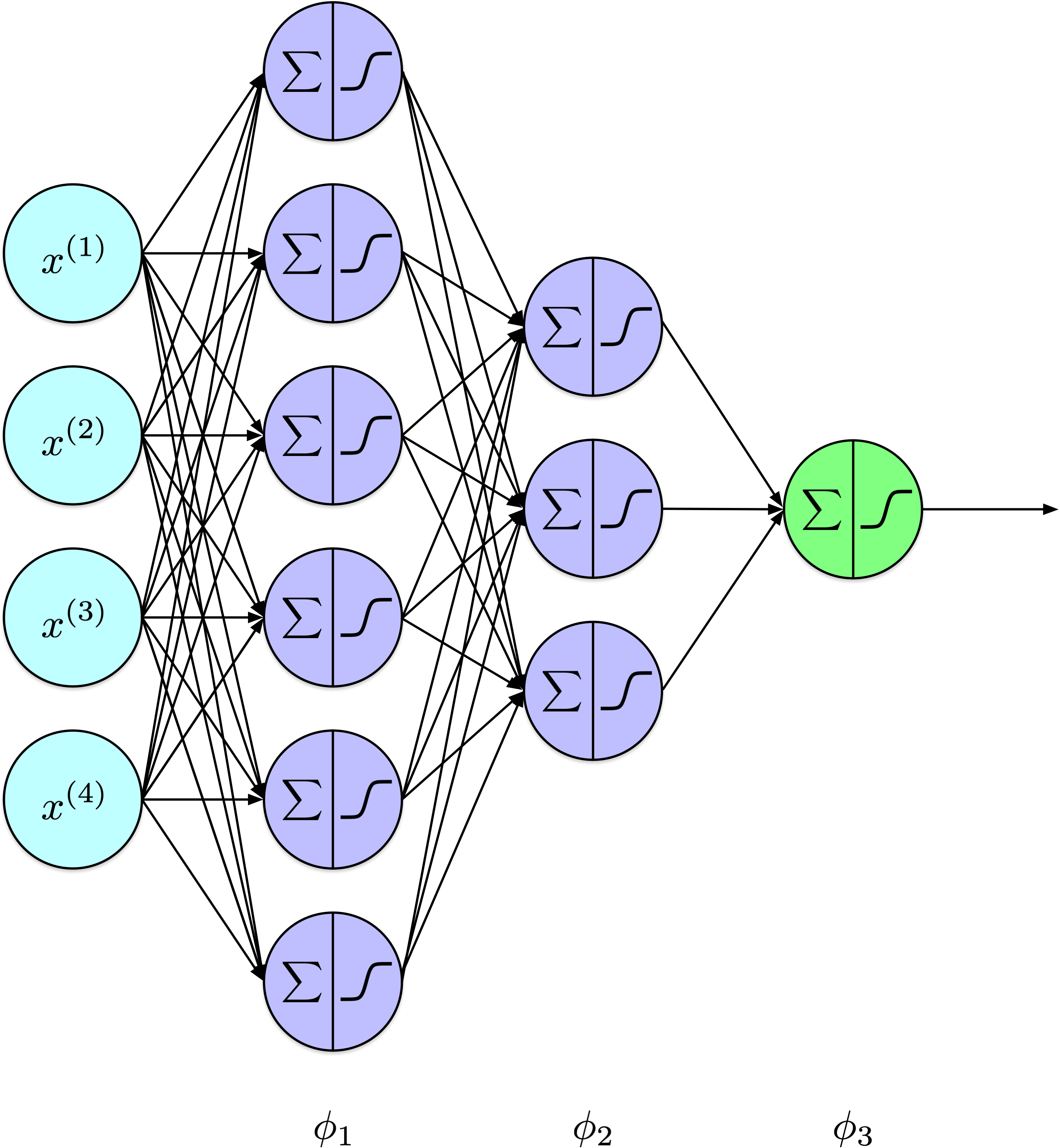
The universal approximation theorem states that a feedforward neural network with a single hidden layer containing a finite number of neurons can approximate any continuous function on a compact subset of \(\mathbb{R}^n\), given appropriate weights and activation functions.

Cybenko (1989); Hornik, Stinchcombe, and White (1989)

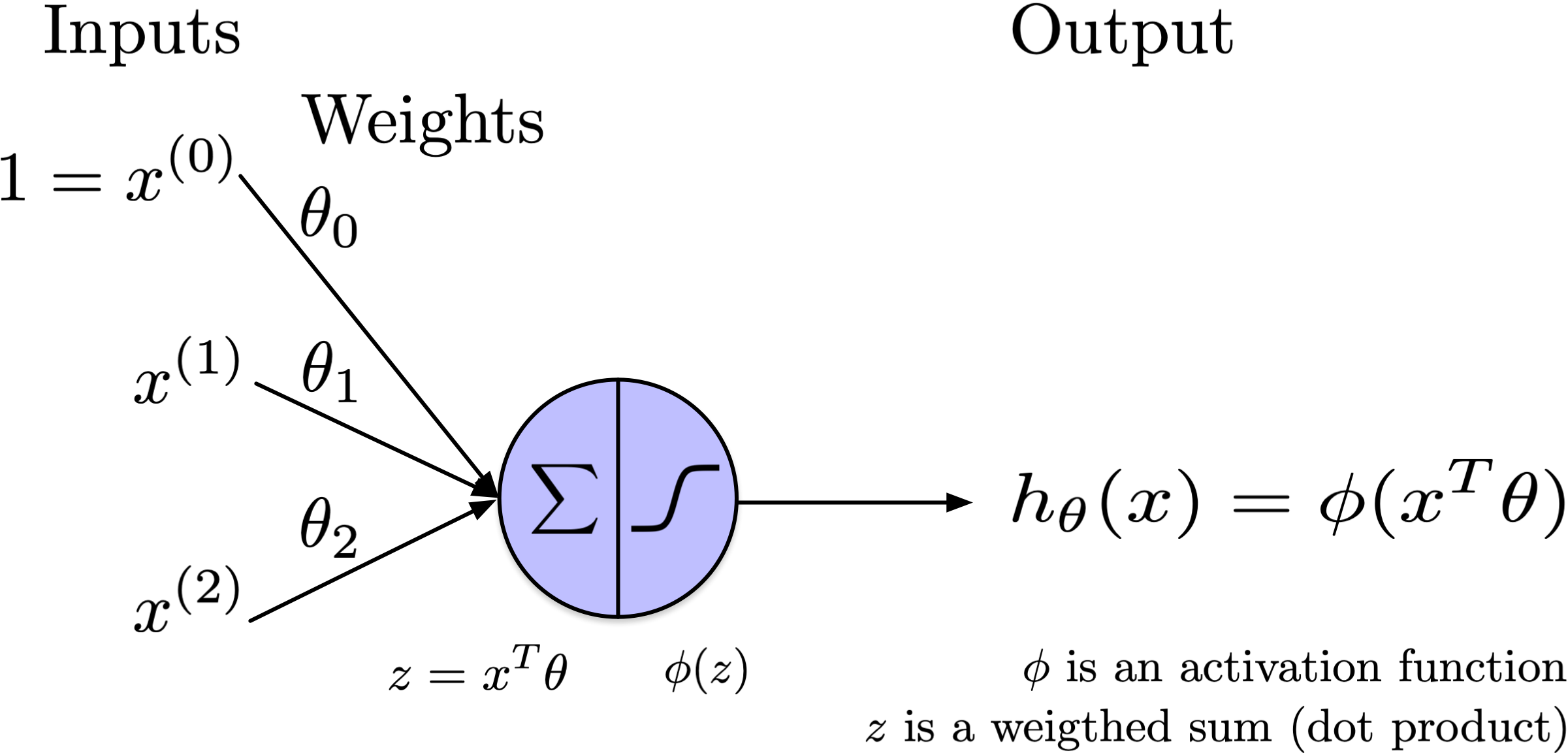
Notation

Notation

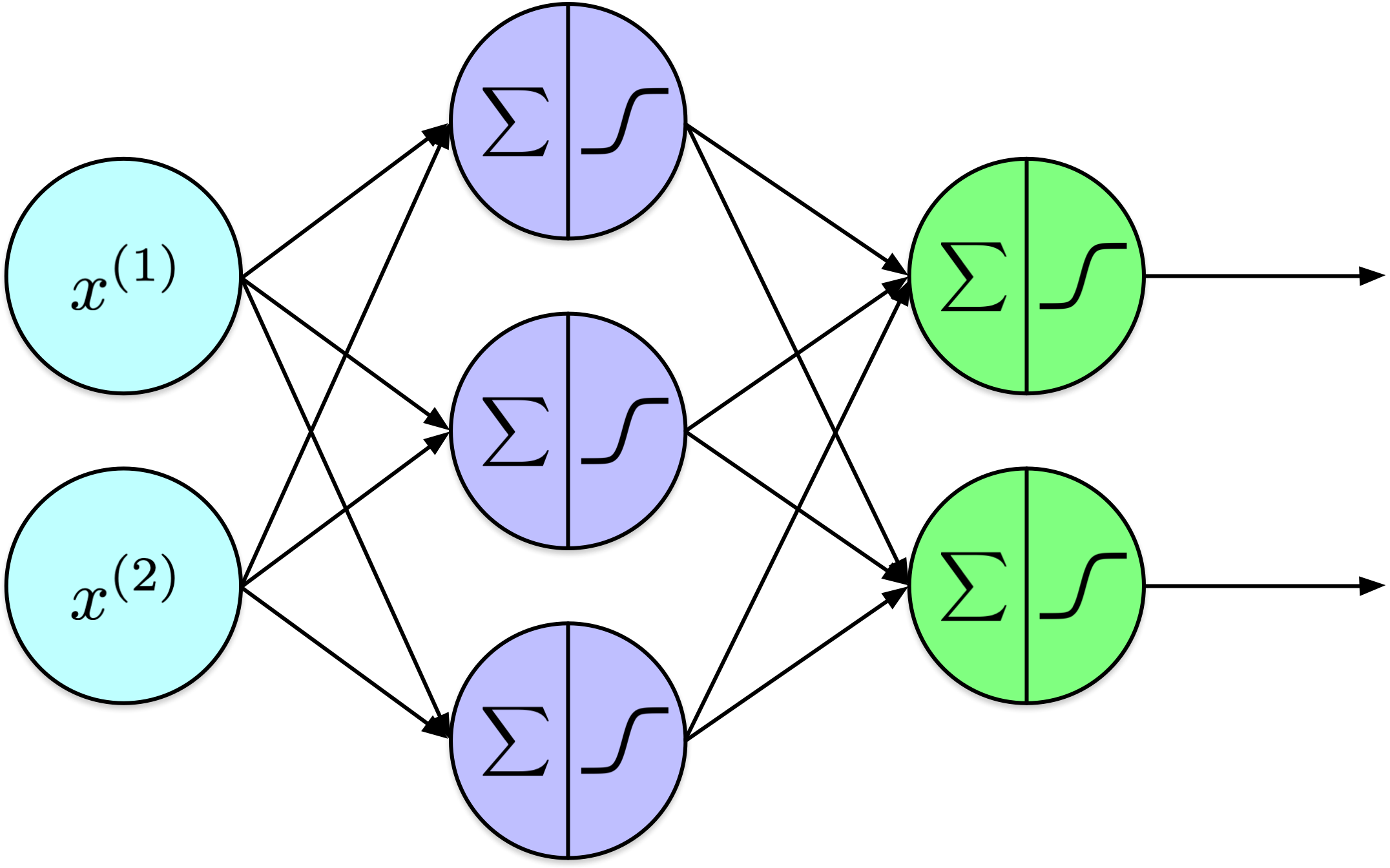
A two-layer perceptron computes:

\[ y = \phi_2(\phi_1(X)) \]

where

\[ \phi_l(Z) = \phi(W_lZ_l + b_l) \]

Where \(\phi\) is an activation function, \(W\) a weight matrix, \(X\) an input matrix, and \(b\) a bias vector.

Notation

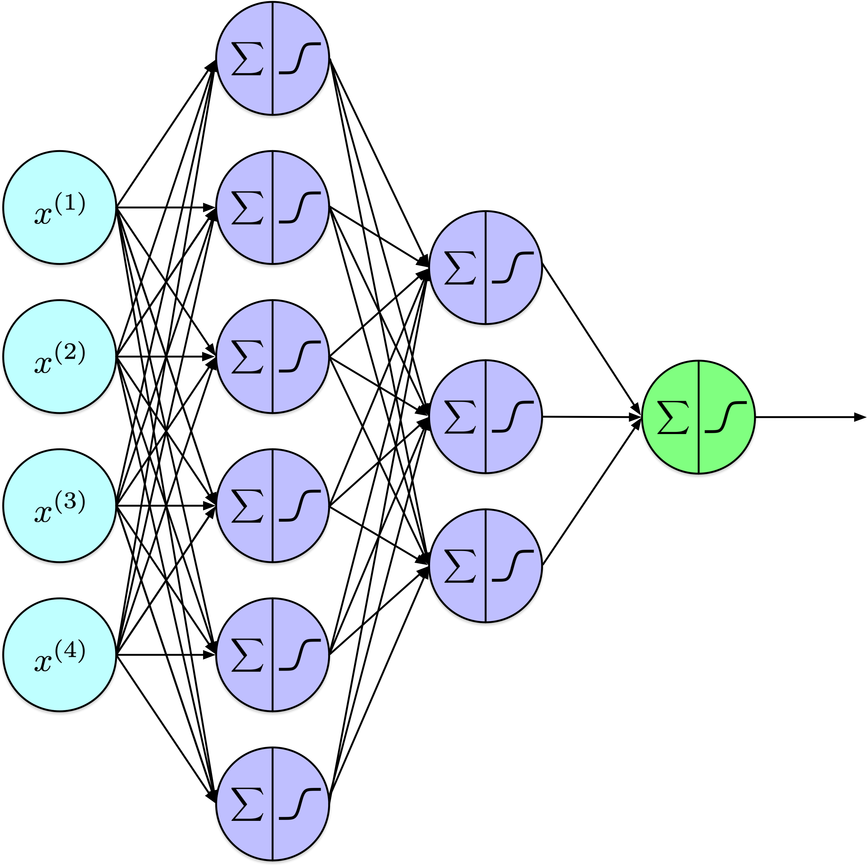
A 3-layer perceptron computes:

\[ y = \phi_3(\phi_2(\phi_1(X))) \]

where

\[ \phi_l(Z) = \phi(W_lZ_l + b_l) \]

Notation

A \(k\)-layer perceptron computes:

\[ y = \phi_k( \ldots \phi_2(\phi_1(X)) \ldots ) \]

where

\[ \phi_l(Z) = \phi(W_lZ_l + b_l) \]

A feedforward network exhibits a consistent structure, where each layer executes the same type of computation on varying inputs. Specifically, the input to layer \(l\) is the output from layer \(l-1\).

Backpropagation

3Blue1Brown

Backpropagation

Learning representations by back-propagating errors

David E. Rumelhart, Geoffrey E. Hinton & Ronald J. Williams

We describe a new learning procedure, back-propagation, for networks of neurone-like units. The procedure repeatedly adjusts the weights of the connections in the network so as to minimize a measure of the difference between the actual output vector of the net and the desired output vector. As a result of the weight adjustments, internal ‘hidden’ units which are not part of the input or output come to represent important features of the task domain, and the regularities in the task are captured by the interactions of these units. The ability to create useful new features distinguishes back-propagation from earlier, simpler methods such as the perceptron-convergence procedure.

I am presenting here the abstract from the seminal Nature publication where Hinton and colleagues introduced the backpropagation algorithm. This abstract is both elegant and informative, effectively capturing the core principles of modern neural networks: the concept of a loss function, the iterative adjustment of weights through the gradient descent algorithm, and the critical role of hidden layers in generating useful task-dependent features.

Nature is a prestigious journal, and it only occasionally publishes content related to computer science.

At the time of this publication, Hinton was affiliated with Carnegie Mellon University. As a reminder, Hinton received the Nobel Prize in Physics in 2024 for his contributions to developing foundational methods in modern machine learning.

The abstract highlights the rationale for using hidden layers in neural networks. The initial hidden layers learn simple representations directly from the input data, while subsequent layers identify associations among these representations. Each layer builds upon the knowledge of previous layers, culminating in the network’s final output.

Rumelhart, Hinton, and Williams (1986)

Before the Backpropagation

• Limitations, such as the inability to solve the XOR classification task, essentially stalled research on neural networks.

• The perceptron was limited to a single layer, and there was no known method for training a multi-layer perceptron.

• Single-layer perceptrons are limited to solving classification tasks that are linearly separable.

Backpropagation: Contributions

• The model employs mean squared error as its loss function.

• Gradient descent is used to minimize loss.

• A sigmoid activation function is used instead of a step function, as its derivative provides valuable information for gradient descent.

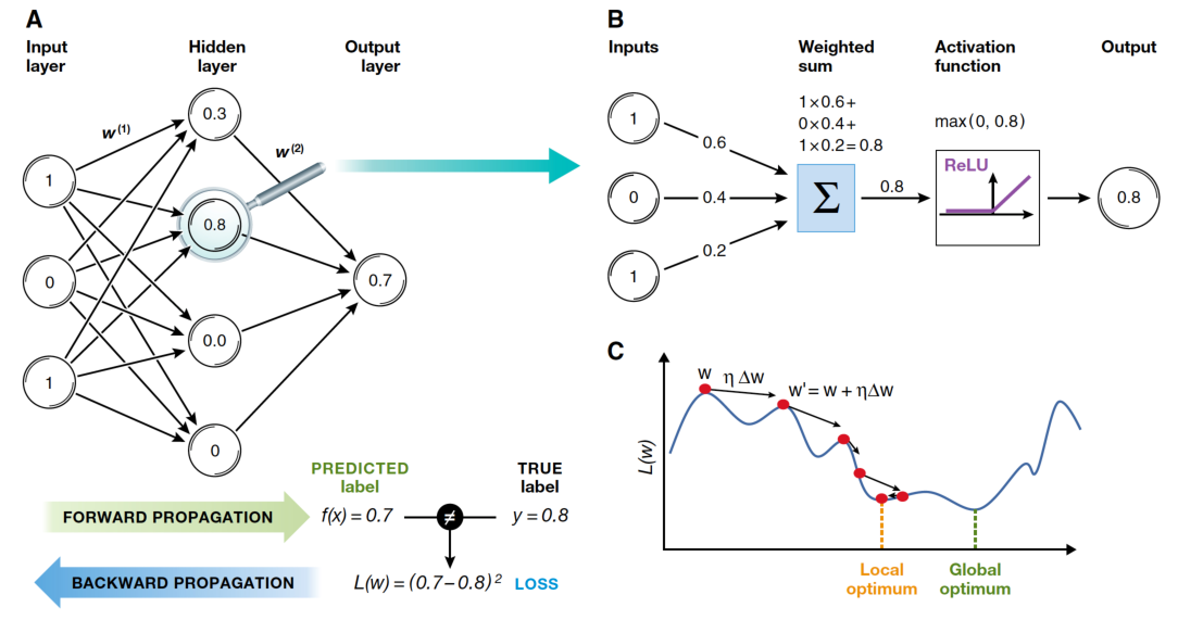
• Shows how updating internal weights using a two-pass algorithm consisting of a forward pass and a backward pass.

• Enables training multi-layer perceptrons.

Backpropagation: Top Level

1. Initialization

2. Forward Pass

3. Compute Loss

4. Backward Pass (Backpropagation)

5. Repeat 2 to 5.

The algorithm stops either after a predefined number of epochs or when convergence criteria are satisfied.

Backpropagation: 1. Initialization

Initialize the weights and biases of the neural network.

1. Zero Initialization
   • All weights are initialized to zero.
   • Symmetry problems, all neurons produce identical outputs, preventing effective learning.
2. Random Initialization
   • Weights are initialized randomly, often using a uniform or normal distribution.
   • Breaks the symmetry between neurons, allowing them to learn.
   • If not scaled properly, leads to slow convergence or vanishing/exploding gradients.

Initializing weights and biases to zero works for logistic regression because it is a linear model with a single layer. In logistic regression, each feature’s weight is independently adjusted during training, and the optimization process can converge correctly regardless of the initial weights, provided the data is linearly separable.

However, zero initialization does not work well for neural networks due to their multi-layered structure. Here’s why:

1. Symmetry Breaking: Neural networks require breaking symmetry between neurons in each layer so that they can learn different features. If all weights are initialized to zero, each neuron in a layer will compute the same output and receive the same gradient during backpropagation. This results in the neurons updating identically, preventing them from learning distinct features and effectively rendering multiple neurons redundant.

2. Non-Linearity: Neural networks rely on non-linear transformations between layers to model complex relationships in the data. Zero initialization inhibits the ability of neurons to activate differently, impeding the network’s capacity to capture non-linear patterns.

See also: Xavier/Glorot and He initialization (later)

Backpropagation: 2. Forward Pass

For each example in the training set (or in a mini-batch):

• Input Layer: Pass input features to first layer.

• Hidden Layers: For each hidden layer, compute the activations (output) by applying the weighted sum of inputs plus bias, followed by an activation function (e.g., sigmoid, ReLU).

• Output Layer: Same process as hidden layers. Output layer activations represent the predicted values.

In practice, it is the mini-batch version of this algorithm that is being used.

The forward pass is almost identical to applying the network for prediction (.predict()), with the exception that intermediate (activation) results are saved, as they are needed for the backward pass.

Backpropagation: 3. Compute Loss

Calculate the loss (error) using a suitable loss function by comparing the predicted values to the actual target values.

A smaller loss indicates that the predicted values are closer to the actual target values.

The value of the loss function can serve as a stopping criterion, with backpropagation halting when the loss is sufficiently small.

Crucially, the derivative of the loss function provides essential information for adjusting the network’s weights and bias terms.

More on the various loss functions coming later: mean squared error for regression tasks or cross-entropy loss for classification tasks.

Backpropagation: 4. Backward Pass

• Output Layer: Compute the gradient of the loss with respect to the output layer’s weights and biases using the chain rule of calculus.

• Hidden Layers: Propagate the error backward through the network, layer by layer. For each layer, compute the gradient of the loss with respect to the weights and biases. Use the derivative of the activation function to help calculate these gradients.

• Update Weights and Biases: Adjust the weights and biases using the calculated gradients and a learning rate, which determines the step size for each update.

At the end of the presentation, links are provided to a series of videos by Herman Kamper. These videos elucidate the intricacies of the backpropagation algorithm across various architectures, both with and without forks, utilizing function composition and graph computation approaches.

While the algorithm is complex due to the numerous cases it entails, its regular structure makes it suitable for automation. Specifically, algorithms like automatic differentiation (autodiff) facilitate this process.

In 1970, Seppo Ilmari Linnainmaa introduced the algorithm known as reverse mode automatic differentiation in his MSc thesis. Although he did not apply this algorithm to neural networks, it is more general than backpropagation.

Common optimization techniques like gradient descent or its variants (e.g., Adam) are employed.

Key Concepts

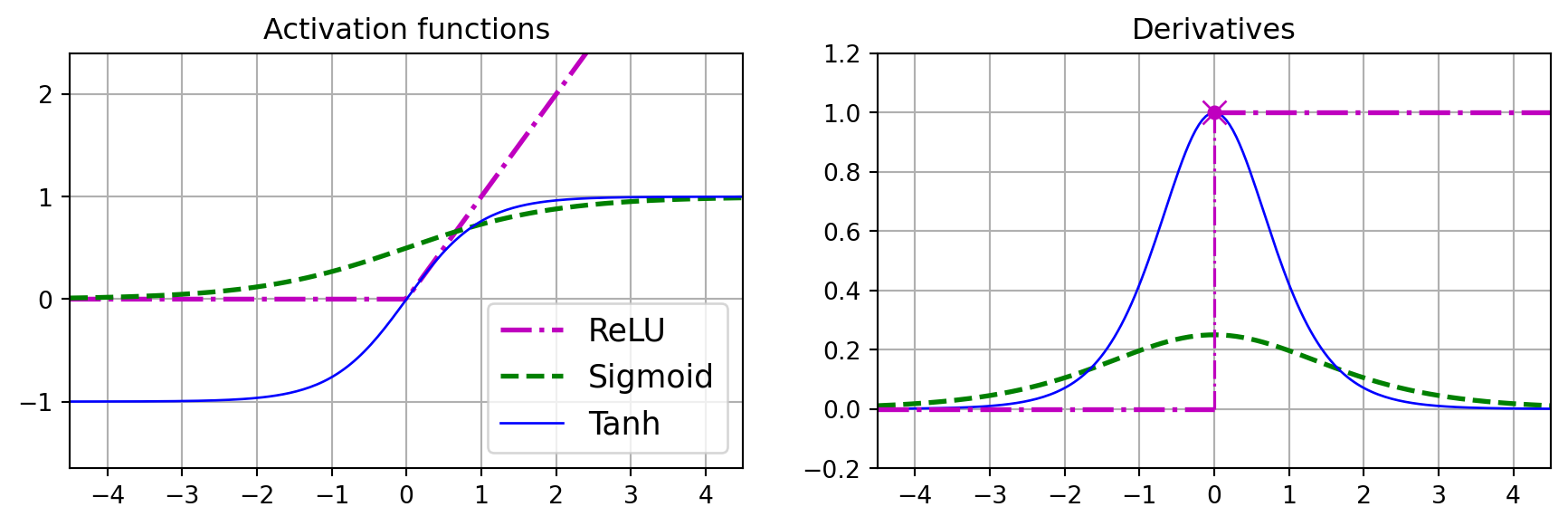
• Activation Functions: Functions like sigmoid, ReLU, and tanh introduce non-linearity, which allows the network to learn complex patterns.

• Learning Rate: A hyperparameter that controls how much to change the model in response to the estimated error each time the model weights are updated.

• Gradient Descent: An optimization algorithm used to minimize the loss function by iteratively moving towards the steepest descent as defined by the negative of the gradient.

Summary

Attribution: Angermueller et al. (2016)

Training

Vanishing Gradients

• Vanishing gradient problem: Gradients become too small, hindering weight updates.

• Stalled neural network research (again) in early 2000s.

• Sigmoid and its derivative (range: 0 to 0.25) were key factors.

• Common initialization: Weights/biases from \(\mathcal{N}(0, 1)\) contributed to the issue.

Glorot and Bengio (2010) shed light on the problems.

The vanishing gradient problem often occurs with activation functions like the sigmoid and hyperbolic tangent (tanh), leading to difficulties in training deep neural networks due to diminishing gradients that slow down learning.

In contrast, the exploding gradient problem, which involves gradients growing excessively large, is typically observed in architectures such as recurrent neural networks (RNNs).

Both issues can significantly affect the stability and convergence of gradient-based optimization techniques, thereby hindering the effective training of deep models.

Vanishing Gradients: Solutions

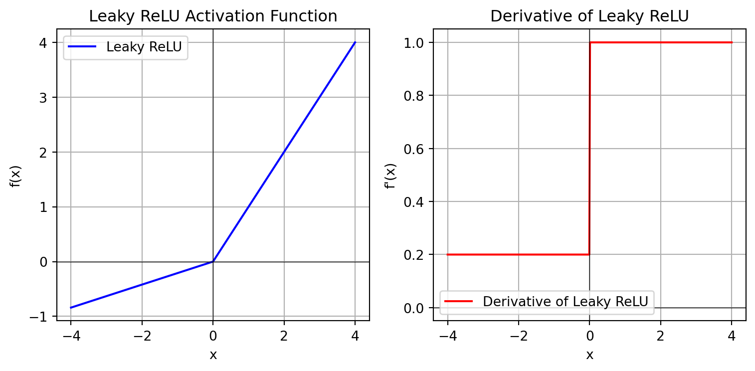
• Alternative activation functions: Rectified Linear Unit (ReLU) and its variants (e.g., Leaky ReLU, Parametric ReLU, and Exponential Linear Unit).

• Weight Initialization: Xavier (Glorot) or He initialization.

Other techniques exists to mitigate the problem, including those:

• Batch Normalization: Implement batch normalization to standardize the inputs to each layer, which can help stabilize and accelerate training by reducing internal covariate shift and maintaining effective gradient flow.

• Residual Networks: Use residual connections, as seen in ResNet architectures, which allow gradients to flow more easily through the network by providing shortcut paths that bypass one or more layers.

He Initialization

A similar but slightly different initialization method design to work with ReLU, as well as Leaky ReLU, ELU, GELU, Swish, and Mish.

Ensure that the initialization method matches the chosen activation function.

import tensorflow as tf
from tensorflow.python.keras.layers import Dense

dense = Dense(50, activation="relu", kernel_initializer="he_normal")

• Glorot Initialization (Xavier Initialization): This method sets the initial weights based on the number of input and output units for each layer, aiming to keep the variance of activations consistent across layers. It is particularly effective for activation functions like sigmoid and tanh.

• He Initialization: This approach adjusts the weight initialization to be suitable for layers using ReLU and its variants, by scaling the variance according to the number of input units only.

AKA Kaiming initialization.

Note

Randomly initializing the weights¹ is sufficient to break symmetry in a neural network, allowing the bias terms to be set to zero without impacting the network’s ability to learn effectively.

1. Proper initialization of weights, such as using Xavier/Glorot or He initialization, is crucial and should be aligned with the choice of activation function to ensure optimal network performance.

Activation Function: Leaky ReLU

import numpy as np
import matplotlib.pyplot as plt

# Define the Leaky ReLU function
def leaky_relu(x, alpha=0.21):
    return np.where(x > 0, x, alpha * x)

# Define the derivative of the Leaky ReLU function
def leaky_relu_derivative(x, alpha=0.2):
    return np.where(x > 0, 1, alpha)

# Generate a range of input values
x_values = np.linspace(-4, 4, 400)

# Compute the Leaky ReLU and its derivative
leaky_relu_values = leaky_relu(x_values)
leaky_relu_derivative_values = leaky_relu_derivative(x_values)

# Create the plot
plt.figure(figsize=(8, 4))

# Plot the Leaky ReLU
plt.subplot(1, 2, 1)
plt.plot(x_values, leaky_relu_values, label='Leaky ReLU', color='blue')
plt.title('Leaky ReLU Activation Function')
plt.xlabel('x')
plt.ylabel('f(x)')
plt.grid(True)
plt.axhline(0, color='black',linewidth=0.5)
plt.axvline(0, color='black',linewidth=0.5)
plt.legend()

# Plot the derivative of the Leaky ReLU
plt.subplot(1, 2, 2)
plt.plot(x_values, leaky_relu_derivative_values, label='Derivative of Leaky ReLU', color='red')
plt.title('Derivative of Leaky ReLU')
plt.xlabel('x')
plt.ylabel("f'(x)")
plt.grid(True)
plt.axhline(0, color='black',linewidth=0.5)
plt.axvline(0, color='black',linewidth=0.5)
plt.legend()

# Show the plots
plt.tight_layout()
plt.show()

When the input to the ReLU activation function, the weighted sum plus bias, is negative for all the training examples, the output value of ReLU is zero. But also, its derivative is 0, which effectively deactivates the neuron. Leaky ReLU, or other variants, effectively mitigates the issue.

import tensorflow as tf
from tensorflow.python.keras.layers import Dense

leaky_relu = tf.keras.layers.LeakyReLU(negative_slope=0.2)
dense = tf.keras.layers.Dense(50, activation=leaky_relu, kernel_initializer="he_normal")

Keras proposes 18 layer activation functions at the time of writing.

The Leaky ReLU, a variant of the standard ReLU activation function, effectively mitigates the issue of dying ReLU nodes. For negative input values, it introduces a linear component with a slope governed by the parameter negative_slope.

Output Layer

Output Layer: Regression Task

• # of output neurons:
  • 1 per dimension
• Output layer activation function:
  • None, ReLU/softplus, if positive, sigmoid/tanh, if bounded
• Loss function:
  • MeanSquaredError

In an object detection problem, determining the bounding box exemplifies a regression task where the output is multidimensional.

Output Layer: Classification Task

• # of output neurons:
  • 1 if binary, 1 per class, if multi-label or multiclass.
• Output layer activation function:
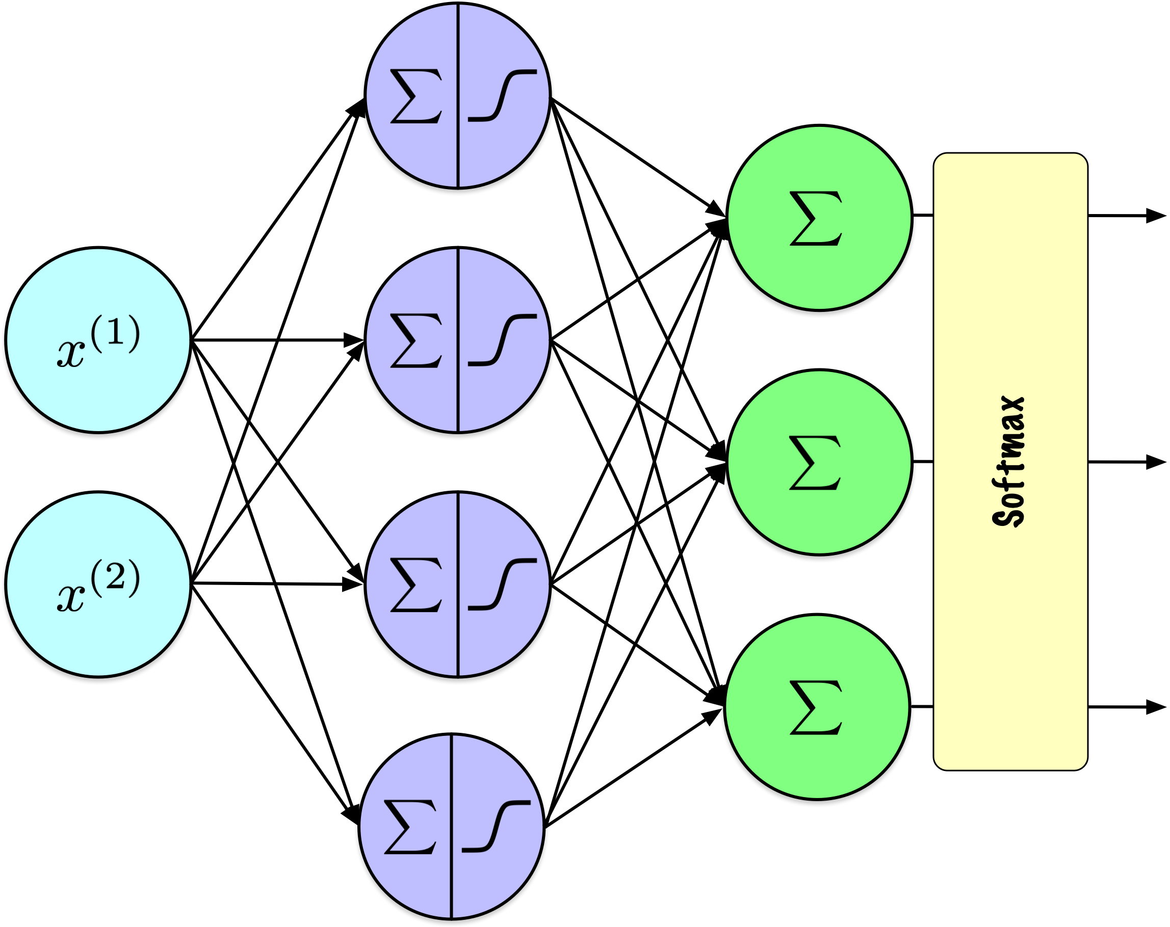
  • sigmoid, if binary or multi-label, softmax if multi-class.
• Loss function:
  • cross-entropy

Softmax

Observe that I have revised the representation of the output nodes to indicate that the softmax function is applied to the entire layer, rather than to individual nodes. This function transforms the raw output values of the layer into probabilities that sum to 1, facilitating multi-class classification. This characteristic distinguishes it from activation functions like ReLU or sigmoid, which are typically applied independently to each node’s output.

The argmax function is not suitable for optimization via gradient-based methods because its derivative is zero in all cases, similar to step functions. In contrast, the softmax function offers both a probabilistic interpretation and a computable derivative, making it more effective for such applications.

The argmax function can be applied a posteriori to trained networks for class prediction.

Softmax ensures that all activation outputs fall between 0 and 1 and collectively sum to 1.

Softmax

The softmax function is an activation function used in multi-class classification problems to convert a vector of raw scores into probabilities that sum to 1.

Given a vector \(\mathbf{z} = [z_1, z_2, \ldots, z_n]\):

\[ \sigma(\mathbf{z})_i = \frac{e^{z_i}}{\sum_{j=1}^{n} e^{z_j}} \]

where \(\sigma(\mathbf{z})_i\) is the probability of the \(i\)-th class, and \(n\) is the number of classes.

Softmax emphasizes higher scores while suppressing lower ones, enabling a probabilistic interpretation of the outputs.

We clearly see that such an activation applies for an entire layer since the denomination depends on the values of all the \(z_j\), for \(j in 1 \ldots n\).

Softmax

\(z_1\)	\(z_2\)	\(z_3\)	\(\sigma(z_1)\)	\(\sigma(z_2)\)	\(\sigma(z_3)\)	\(\sum\)
1.47	-0.39	0.22	0.69	0.11	0.20	1.00
5.00	6.00	4.00	0.24	0.67	0.09	1.00
0.90	0.80	1.10	0.32	0.29	0.39	1.00
-2.00	2.00	-3.00	0.02	0.98	0.01	1.00

1. Maintains Relative Order: The softmax function preserves the relative order of the input values. If one input is greater than another, its corresponding output will also be greater.

2. Interpreted as probabilities: Each value is in the range 0 to 1. The output values from the softmax function are normalized to sum to one, which allows them to be interpreted as probabilities.

3. Relative Differences: When the relative differences among the input values are small, the differences in the output probabilities remain small, reflecting the input distribution. When the input values are identical, the output values will be \(\frac{1}{n}\), where \(n\) is the number of classes.

4. Wide Range of Values: The softmax function can effectively handle a wide range of input values, thanks to the exponential function and normalization, which scale the inputs to a probabilistic range.

These properties make the softmax function particularly useful for multi-class classification tasks in machine learning.

Softmax values for a vector of length 3.

Softmax

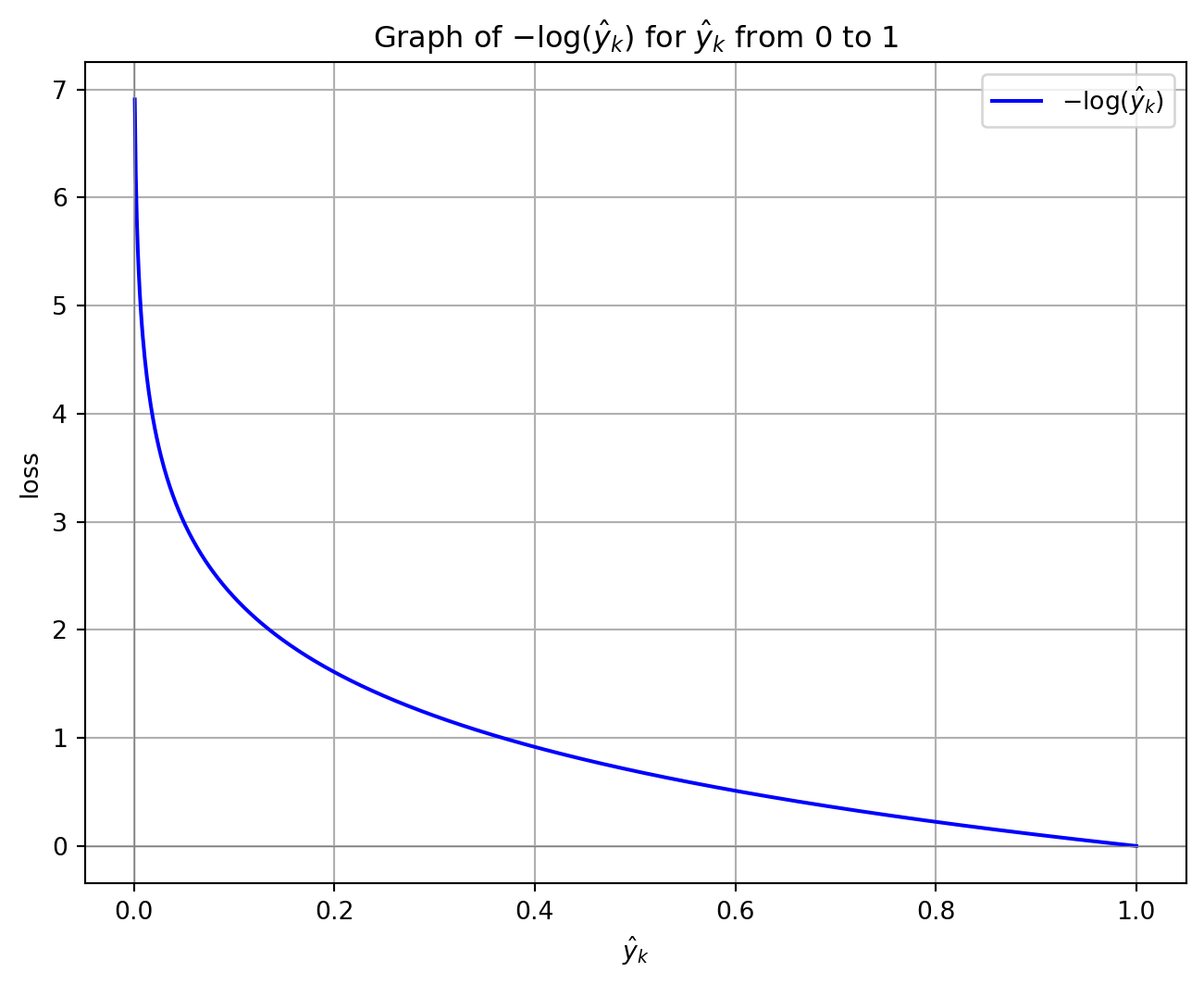
Cross-entropy loss function

The cross-entropy in a multi-class classification task for one example:

\[ J(W) = -\sum_{k=1}^{K} y_k \log(\hat{y}_k) \]

Where:

• \(K\) is the number of classes.
• \(y_k\) is the true distribution for the class \(k\).
• \(\hat{y}_k\) is the predicted probability of class \(k\) from the model.

• The target vector \(y\) is expressed as a one-hot encoded vector of length \(K\), where the element corresponding to the true class is set to 1, and all other elements are 0.

• Consequently, in the summation over classes, only the term associated with the true class contributes a non-zero value.

• Therefore, the cross-entropy loss for a single example is given by \(-\log(\hat{y}_k)\), where \(\hat{y}_k\) is the predicted probability for the true class.

• The predicted probability \(\hat{y}_k\) is derived from the softmax function applied in the output layer of the neural network.

Cross-entropy loss function

• Classification Problem: 3 classes
  • Versicolour, Setosa, Virginica.
• One-Hot Encoding:
  • Setosa = \([0, 1, 0]\).
• Softmax Outputs & Loss:
  • \([0.22,\mathbf{0.7}, 0.08]\): Loss = \(-\log(0.7) = 0.3567\).
  • \([0.7, \mathbf{0.22}, 0.08]\): Loss = \(-\log(0.22) = 1.5141\).
  • \([0.7, \mathbf{0.08}, 0.22]\): Loss = \(-\log(0.08) = 2.5257\).

Among the softmax outputs, cross-entropy evaluates only the component corresponding to \(k=1\) (Setosa), as the other entries in the one-hot encoded vector are zero. This relevant element is highlighted in bold. When the softmax prediction aligns closely with the expected value, the resulting loss is minimal (0.3567). Conversely, as the prediction deviates further from the expected value, the loss increases (1.5141 and 2.5257).

Case: one example

import numpy as np
import matplotlib.pyplot as plt

# Generate an array of p values from just above 0 to 1
p_values = np.linspace(0.001, 1, 1000)

# Compute the natural logarithm of each p value
ln_p_values = - np.log(p_values)

# Plot the graph
plt.figure(figsize=(8, 6))
plt.plot(p_values, ln_p_values, label=r'$-\log(\hat{y}_k)$', color='b')

# Add labels and title
plt.xlabel(r'$\hat{y}_k$')
plt.ylabel(r'loss')
plt.title(r'Graph of $-\log(\hat{y}_k)$ for $\hat{y}_k$ from 0 to 1')
plt.grid(True)
plt.axhline(0, color='gray', lw=0.5)  # Add horizontal line at y=0
plt.axvline(0, color='gray', lw=0.5)  # Add vertical line at x=0

# Display the plot
plt.legend()
plt.show()

• In the summation, only the term where \(y_k = 1\) contributes a non-zero value.

• Due to the negative sign preceding the summation, the value of the function is \(-\log(\hat{y}_k\).

• If the predicted probability \(\hat{y}_k\) is near 1, the loss approaches zero, indicating minimal penalty.

• Conversely, as \(\hat{y}_k\) nears 0, indicating an incorrect prediction, the loss approaches infinity. This substantial penalty allows cross-entropy loss to converge more quickly than mean squared error.

Case: Dataset

For a dataset with \(N\) examples, the average cross-entropy loss over all examples is computed as:

\[ L = -\frac{1}{N} \sum_{i=1}^{N} \sum_{k=1}^{K} y_{i,k} \log(\hat{y}_{i,k}) \]

Where:

• \(i\) indexes over the different examples in the dataset.
• \(y_{i,k}\) and \(\hat{y}_{i,k}\) are the true and predicted probabilities for class \(k\) of example \(i\), respectively.

Regularization

Definition

Regularization comprises a set of techniques designed to enhance a model’s ability to generalize by mitigating overfitting. By discouraging excessive model complexity, these methods improve the model’s robustness and performance on unseen data.

Adding penalty terms to the loss

• In numerical optimization, it is standard practice to incorporate additional terms into the objective function to deter undesirable model characteristics.

• For a minimization problem, the optimization process aims to circumvent the substantial costs associated with these penalty terms.

Loss Function

Consider the mean absolute error loss function:

\[ \mathrm{MAE}(X,W) = \frac{1}{N} \sum_{i=1}^N | h_W(x_i) - y_i | \]

Where:

• \(W\) are the weights of our network.
• \(h_W(x_i)\) is the output of the network for example \(i\).
• \(y_i\) is the true label for example \(i\).

Penalty Term(s)

One or more terms can be added to the loss:

\[ \mathrm{MAE}(X,W) = \frac{1}{N} \sum_{i=1}^N | h_W(x_i) - y_i | + \mathrm{penalty} \]

Norm

A norm is assigns a non-negative length to a vector.

The \(\ell_p\) norm of a vector \(\mathbf{z} = [z_1, z_2, \ldots, z_n]\) is defined as:

\[ \|\mathbf{z}\|_p = \left( \sum_{i=1}^{n} |z_i|^p \right)^{1/p} \]

A norm is a function that assigns a non-negative length or size to each vector in a vector space, satisfying certain properties: positivity, scalar multiplication, the triangle inequality, and the property that the norm is zero if and only if the vector is zero.

With larger \(p\), the \(\ell_p\) norm increasingly highlights larger \(z_i\) values due to exponentiation.

\(\ell_1\) and \(\ell_2\) norms

The \(\ell_1\) norm (Manhattan norm) is:

\[ \|\mathbf{z}\|_1 = \sum_{i=1}^{n} |z_i| \]

The \(\ell_2\) norm (Euclidean norm) is:

\[ \|\mathbf{z}\|_2 = \sqrt{\sum_{i=1}^{n} z_i^2} \]

\(\ell_1\) and \(\ell_2\) regularization

Below, \(\alpha\) and \(\beta\) determine the degree of regularization applied; setting these values to zero effectively disables the regularization term.

\[ \mathrm{MAE}(X,W) = \frac{1}{N} \sum_{i=1}^N | h_W(x_i) - y_i | + \alpha \ell_1 + \beta \ell_2 \]

Guidelines

• \(\ell_1\) Regularization:
  • Promotes sparsity, setting many weights to zero.
  • Useful for feature selection by reducing feature reliance.
• \(\ell_2\) Regularization:
  • Promotes small, distributed weights for stability.
  • Ideal when all features contribute and reducing complexity is key.

Keras Example

import tensorflow as tf
from tensorflow.python.keras.layers import Dense

regularizer = tf.keras.regularizers.l2(0.001)

dense = Dense(50, kernel_regularizer=regularizer)

This layer specifically utilizes \(\ell_2\) regularization, in contrast to the prior discussion where regularization was applied globally across the entire model.

Dropout

Dropout is a regularization technique in neural networks where randomly selected neurons are ignored during training, reducing overfitting by preventing co-adaptation of features.

Hinton et al. (2012)

Dropout

• During each training step, each neuron in a dropout layer has a probability \(p\) of being excluded from the computation, typical values for \(p\) are between 10% and 50%.

• While seemingly counterintuitive, this approach prevents the network from depending on specific neurons, promoting the distribution of learned representations across multiple neurons.

Dropout

• Dropout is one of the most popular and effective methods for reducing overfitting.

• The typical improvement in performance is modest, usually around 1 to 2%.

Keras

import keras
from keras.models import Sequential
from keras.layers import InputLayer, Dropout, Flatten, Dense

model = tf.keras.Sequential([
    InputLayer(shape=[28, 28]),
    Flatten(),
    Dropout(rate=0.2),
    Dense(300, activation="relu"),
    Dropout(rate=0.2),
    Dense(100, activation="relu"),
    Dropout(rate=0.2),
    Dense(10, activation="softmax")
])

The dropout rate may differ between layers; larger rates can be applied to larger layers, while smaller rates are suitable for smaller layers. It is common practice in many networks to apply dropout only after the final hidden layer.

Adding Dropout layers to the Fashion-MNIST model from last lecture.

Definition

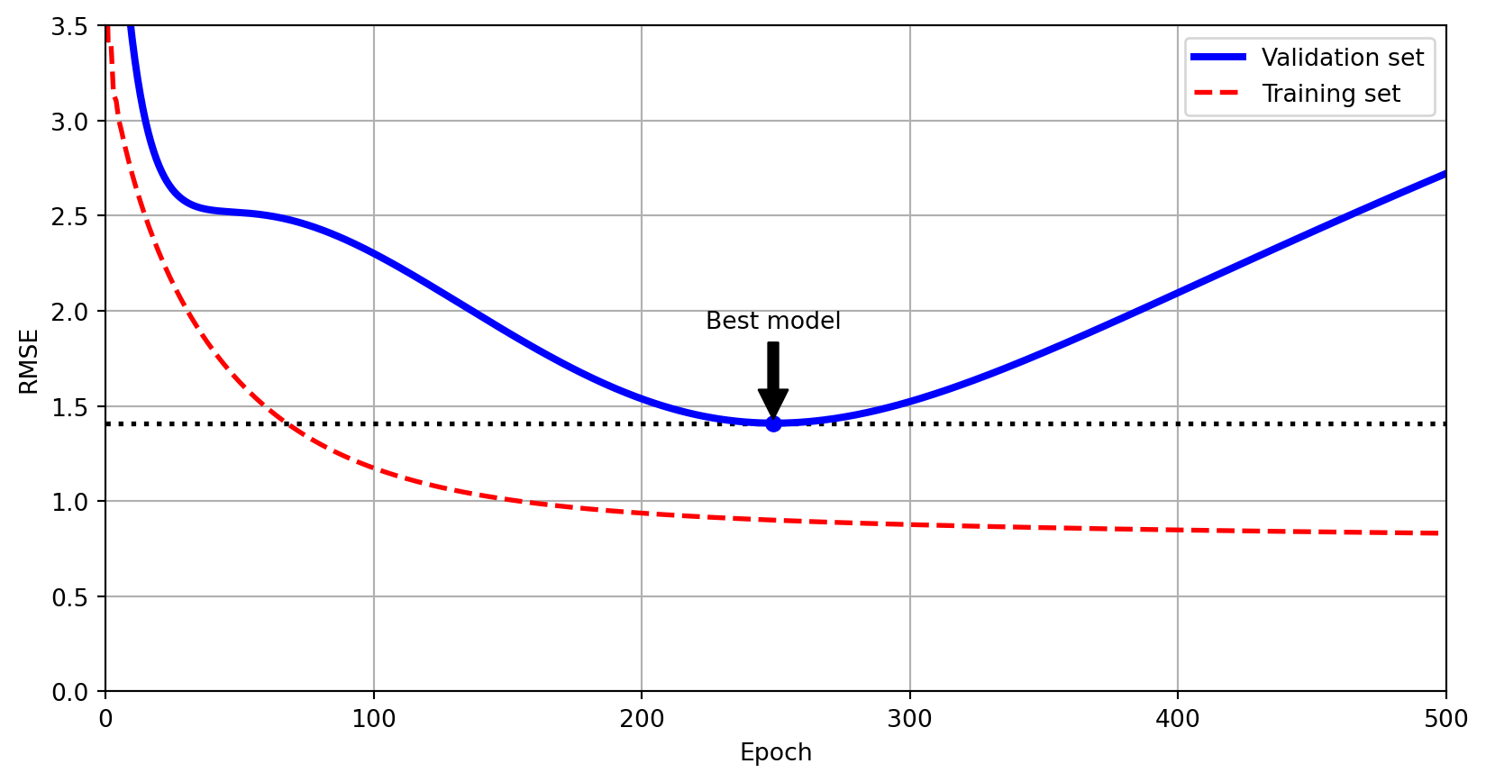
Early stopping is a regularization technique that halts training once the model’s performance on a validation set begins to degrade, preventing overfitting by stopping before the model learns noise.

Geoffrey Hinton calls this the “beautiful free lunch.”

Early Stopping

from copy import deepcopy
from sklearn.metrics import root_mean_squared_error
from sklearn.preprocessing import StandardScaler
from sklearn.pipeline import make_pipeline
from sklearn.preprocessing import PolynomialFeatures
from sklearn.linear_model import SGDRegressor

# extra code – creates the same quadratic dataset as earlier and splits it
np.random.seed(42)
m = 100
X = 6 * np.random.rand(m, 1) - 3
y = 0.5 * X ** 2 + X + 2 + np.random.randn(m, 1)
X_train, y_train = X[: m // 2], y[: m // 2, 0]
X_valid, y_valid = X[m // 2 :], y[m // 2 :, 0]

preprocessing = make_pipeline(PolynomialFeatures(degree=90, include_bias=False),
                              StandardScaler())
X_train_prep = preprocessing.fit_transform(X_train)
X_valid_prep = preprocessing.transform(X_valid)
sgd_reg = SGDRegressor(penalty=None, eta0=0.002, random_state=42)
n_epochs = 500
best_valid_rmse = float('inf')
train_errors, val_errors = [], []  # extra code – it's for the figure below

for epoch in range(n_epochs):
    sgd_reg.partial_fit(X_train_prep, y_train)
    y_valid_predict = sgd_reg.predict(X_valid_prep)
    val_error = root_mean_squared_error(y_valid, y_valid_predict)
    if val_error < best_valid_rmse:
        best_valid_rmse = val_error
        best_model = deepcopy(sgd_reg)

    # extra code – we evaluate the train error and save it for the figure
    y_train_predict = sgd_reg.predict(X_train_prep)
    train_error = root_mean_squared_error(y_train, y_train_predict)
    val_errors.append(val_error)
    train_errors.append(train_error)

# extra code – this section generates and saves Figure 4–20
best_epoch = np.argmin(val_errors)
plt.annotate('Best model',
             xy=(best_epoch, best_valid_rmse),
             xytext=(best_epoch, best_valid_rmse + 0.5),
             ha="center",
             arrowprops=dict(facecolor='black', shrink=0.05))
plt.plot([0, n_epochs], [best_valid_rmse, best_valid_rmse], "k:", linewidth=2)
plt.plot(val_errors, "b-", linewidth=3, label="Validation set")
plt.plot(best_epoch, best_valid_rmse, "bo")
plt.plot(train_errors, "r--", linewidth=2, label="Training set")
plt.legend(loc="upper right")
plt.xlabel("Epoch")
plt.ylabel("RMSE")
plt.axis([0, n_epochs, 0, 3.5])
plt.grid()
plt.show()

Attribution: Géron (2022), 04_training_linear_models.ipynb.

Prologue

Summary

• Introduction to Deep Learning in Bioinformatics: Overview of models and repositories like Kipoi, Hugging Face, and DragoNN.
• Neural Network Fundamentals: Discussion of network layers, activation functions (e.g., sigmoid, tanh, ReLU, Leaky ReLU, softmax), and the universal approximation theorem.
• Notation and Architecture: Detailed explanation of how multi-layer perceptrons and feedforward networks are structured and notated.
• Training Mechanics: Step-by-step breakdown of forward propagation, loss computation, and backpropagation using gradient descent.
• Challenges and Solutions: Exploration of issues such as vanishing/exploding gradients and methods to mitigate them (e.g., proper initialization, dropout, early stopping).
• Practical Code Examples and Visualizations: Demonstrations using Keras and TensorFlow to illustrate the concepts in action.

3Blue1Brown

It is highly recommended that you watch this video. While it covers the concepts we have already explored, it presents the material in a manner that is challenging to replicate in a classroom setting.

• Provides a clear explanation of the intuition behind the effectiveness of neural networks, detailing the hierarchy of concepts briefly mentioned in the last lecture.
• Offers a compelling rationale for the necessity of a bias term.
• Similarly, elucidates the concept of activation functions and the importance of a squashing function.
• The segment beginning at 13m 26s offers a visual explanation of the linear algebra involved: \(\sigma(W X^T + b)\).

In my opinion, this is an excellent and informative video.

3Blue1Brown

A series of videos, with animations, providing the intuition behind the backpropagation algorithm.

• Neural networks (playlist)

  • What is backpropagation really doing? (12m 47s)
  • Backpropagation calculus (10m 18s)

Prerequisite: Gradient descent, how neural networks learn? (20m 33s)

StatQuest

• Neural Networks Pt. 2: Backpropagation Main Ideas (17m 34s)
• Backpropagation Details Pt. 1: Optimizing 3 parameters simultaneously (18m 32s)
• Backpropagation Details Pt. 2: Going bonkers with The Chain Rule (13m 9s)

Prerequisites: The Chain Rule (18m 24s) & Gradient Descent, Step-by-Step (23m 54s)

Herman Kamper

One of the most thorough series of videos on the backpropagation algorithm.

• Introduction to neural networks (playlist)

  • Backpropagation (without forks) (31m 1s)
  • Backprop for a multilayer feedforward neural network (4m 2s)
  • Computational graphs and automatic differentiation for neural networks (6m 56s)
  • Common derivatives for neural networks (7m 18s)
  • A general notation for derivatives (in neural networks) (7m 56s)
  • Forks in neural networks (13m 46s)
  • Backpropagation in general (now with forks) (3m 42s)

Next lecture

• Deap Learning Architectures

References

Angermueller, Christof, Tanel Pärnamaa, Leopold Parts, and Oliver Stegle. 2016. “Deep Learning for Computational Biology.” Mol Syst Biol 12 (7): 878. https://doi.org/10.15252/msb.20156651.

Avsec, Ziga, Roman Kreuzhuber, Johnny Israeli, Nancy Xu, Jun Cheng, Avanti Shrikumar, Abhimanyu Banerjee, et al. 2019. “The Kipoi Repository Accelerates Community Exchange and Reuse of Predictive Models for Genomics.” Nature Biotechnology 37 (6): 592–600. https://doi.org/10.1038/s41587-019-0140-0.

Cybenko, George V. 1989. “Approximation by Superpositions of a Sigmoidal Function.” Mathematics of Control, Signals and Systems 2: 303–14. https://api.semanticscholar.org/CorpusID:3958369.

Géron, Aurélien. 2022. Hands-on Machine Learning with Scikit-Learn, Keras, and TensorFlow. 3rd ed. O’Reilly Media, Inc.

Glorot, Xavier, and Yoshua Bengio. 2010. “Understanding the Difficulty of Training Deep Feedforward Neural Networks.” In Proceedings of the Thirteenth International Conference on Artificial Intelligence and Statistics, edited by Yee Whye Teh and Mike Titterington, 9:249–56. Proceedings of Machine Learning Research. Chia Laguna Resort, Sardinia, Italy: PMLR. https://proceedings.mlr.press/v9/glorot10a.html.

He, Kaiming, Xiangyu Zhang, Shaoqing Ren, and Jian Sun. 2016. “Deep Residual Learning for Image Recognition.” In 2016 IEEE Conference on Computer Vision and Pattern Recognition (CVPR), 770–78. https://doi.org/10.1109/CVPR.2016.90.

Hinton, Geoffrey E., Nitish Srivastava, Alex Krizhevsky, Ilya Sutskever, and Ruslan Salakhutdinov. 2012. “Improving Neural Networks by Preventing Co-Adaptation of Feature Detectors.” CoRR abs/1207.0580. http://arxiv.org/abs/1207.0580.

Hornik, Kurt, Maxwell Stinchcombe, and Halbert White. 1989. “Multilayer Feedforward Networks Are Universal Approximators.” Neural Networks 2 (5): 359–66. https://doi.org/https://doi.org/10.1016/0893-6080(89)90020-8.

Rumelhart, David E., Geoffrey E. Hinton, and Ronald J. Williams. 1986. “Learning representations by back-propagating errors.” Nature 323 (6088): 533–36. https://doi.org/10.1038/323533a0.

Marcel Turcotte

Marcel.Turcotte@uOttawa.ca

School of Electrical Engineering and Computer Science (EECS)

University of Ottawa