import numpy as np
import pandas as pd

import matplotlib.pyplot as plt
import seaborn as sns

import networkx as nx

from scipy.stats import multivariate_normal

from sklearn.preprocessing import StandardScaler
from sklearn.model_selection import train_test_split
from sklearn.metrics import classification_report

import tensorflow as tf
from tensorflow import keras
from tensorflow.keras import layersA graph-embedded deep feedforward network for disease outcome classification and feature selection using gene expression data
CSI 5180 - Machine Learning for Bioinformatics
In this notebook, we aim to partially replicate the study conducted by Kong & Yu:
- Kong, Y. & Yu, T. (2018). A graph-embedded deep feedforward network for disease outcome classification and feature selection using gene expression data. Bioinformatics (Oxford, England), 34(21), 3727–3737.
We focus on synthetic data, implement a graph-embedded deep feedforward network using Keras, as well as a baseline model.
Summary of Work
- Gene expression data poses a challenge in predictive modeling due to the small number of samples compared to the large number of features.
- This disparity, known as the ‘n << p’ problem, hinders the application of deep learning techniques for disease outcome classification.
- Sparse learning using external gene network information is a potential solution but remains challenging due to the vast number of features and limited training samples.
- The scale-free structure of gene networks complicates the use of convolutional neural networks.
- Kong & Yu proposed a Graph-Embedded Deep Feedforward Networks (GEDFN) integrating external relational information into deep neural network architecture.
Prepration
This section regroups all the necessary import statements.
Synthetic data generation
Gene expression data is produced under the assumption that the expression levels of adjacent genes within a gene network exhibit correlation.
First, a scale-free graph is generated using the preferential attachment algorithm proposed by Barabási–Albert.
Let’s generate and visualize a small network.
p = 50  # number of features (genes)
m = 1   # number of edges to attach from a new node to existing nodes.

G = nx.barabasi_albert_graph(p, m, seed=42)

pos = nx.spring_layout(G, k=0.1, iterations=100)  # Adjust k as needed
plt.figure(figsize=(12, 12))
nx.draw(G, pos, node_size=10, with_labels=True, labels={node: node for node in G.nodes()})
plt.show()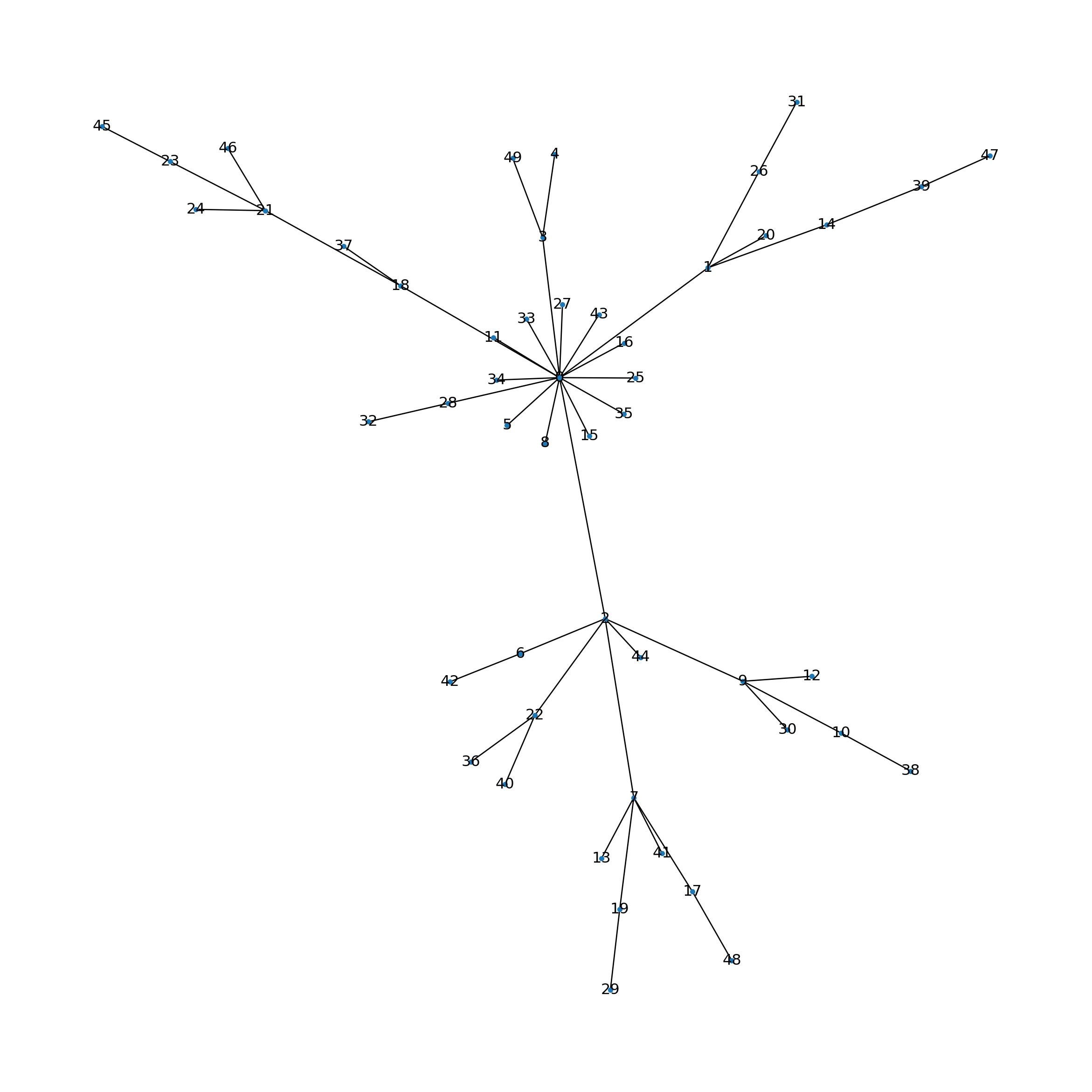
Analogous to biological networks, certain nodes exhibit a high degree of connectivity, thereby forming hubs.
We will now implement the necessary functions for generating gene expression data, grounded in a graph framework and the previously outlined assumptions.
def generate_scale_free_graph(p, m=1):
    """
    Generate a scale-free graph using the Barabási–Albert model.

    Args:
        p (int): Number of nodes (features).
        m (int): Number of edges to attach from a new node to existing nodes.

    Returns:
        G (networkx.Graph): A scale-free network.
    """
    G = nx.barabasi_albert_graph(p, m, seed=42)
    return G

def compute_distance_matrix(G):
    """
    Compute the pairwise shortest-path distance matrix D for graph G.

    Args:
        G (networkx.Graph): The feature graph.

    Returns:
        D (np.ndarray): A (p x p) matrix of shortest-path distances.
    """
    p = G.number_of_nodes()
    D = np.zeros((p, p))
    for i in range(p):
        lengths = nx.single_source_shortest_path_length(G, i)
        for j in range(p):
            D[i, j] = lengths.get(j, np.inf)
    return D

def generate_covariance_matrix(D, decay=0.7):
    """
    Generate a covariance matrix R from the distance matrix D.

    Args:
        D (np.ndarray): Distance matrix.
        decay (float): Decay factor; R[i,j] = decay^(D[i,j]).

    Returns:
        R (np.ndarray): Covariance matrix.
    """
    R = np.power(decay, D)
    np.fill_diagonal(R, 1.0)
    return R

def select_true_predictors(G, p0, s0=0.0):
    """
    Select true predictors based on the feature graph.

    The method selects nodes with high degree (cores) and includes some of their neighbors.

    Args:
        G (networkx.Graph): Feature graph.
        p0 (int): Total number of true predictors to select.
        s0 (float): Proportion of 'singletons' amongst the true predictors.

    Returns:
        true_idx (np.ndarray): Array of indices for true predictors.
    """
    degrees = dict(G.degree())
    # Sort nodes by degree (highest first)
    sorted_nodes = sorted(degrees.items(), key=lambda x: x[1], reverse=True)

    # Choose cores: for example, choose k = max(1, p0//20) top nodes
    k = max(1, p0 // 20)
    cores = [node for node, deg in sorted_nodes[:k]]

    # Determine the number of singletons
    nb_singletons = int(np.ceil(s0 * p0))

    # Remove singletons from the total number of predictors
    p0 -= nb_singletons

    true_predictors = set(cores)
    # Add neighbors of each core until we have p0 predictors
    for core in cores:
        neighbors = list(G.neighbors(core))
        np.random.shuffle(neighbors)
        for neighbor in neighbors:
            if len(true_predictors) < p0:
                true_predictors.add(neighbor)
            else:
                break
        if len(true_predictors) >= p0:
            break
    # If not enough, add additional high-degree nodes
    for node, deg in sorted_nodes:
        if len(true_predictors) < p0:
            true_predictors.add(node)
        else:
            break

    while nb_singletons > 0:
        singleton = np.random.choice(list(G.nodes()))
        if singleton not in true_predictors:
            true_predictors.add(singleton)
            nb_singletons -= 1

    true_idx = np.array(list(true_predictors))[:p0]
    return true_idx

def generate_outcome(X, true_idx, b_range=(0.1, 0.2), threshold=0.5, link='sigmoid'):
    """
    Generate binary outcome variables using a generalized linear model.

    Args:
        X (np.ndarray): Input data matrix (n x p).
        true_idx (np.ndarray): Indices of true predictors.
        b_range (tuple): Range for sampling coefficients.
        threshold (float): Threshold for converting probabilities to binary outcomes.
        link (str): Link function ('sigmoid' or 'tanh_quad').

    Returns:
        y (np.ndarray): Binary outcome vector (n,).
        b (np.ndarray): Coefficients for true predictors.
        b0 (float): Intercept.
        prob (np.ndarray): Computed probabilities.
    """
    p0 = len(true_idx)
    # Sample coefficients uniformly from b_range
    b = np.random.uniform(b_range[0], b_range[1], size=p0)
    # Randomly flip signs (to allow both positive and negative effects)
    signs = np.random.choice([-1, 1], size=p0)
    b = b * signs
    b0 = np.random.uniform(b_range[0], b_range[1])

    # Compute linear combination for each sample
    linear_term = np.dot(X[:, true_idx], b) + b0

    if link == 'sigmoid':
        prob = 1 / (1 + np.exp(linear_term)) # MT: was np.exp(-linear_term)
    elif link == 'tanh_quad':
        # Example non-monotone function: weighted tanh plus quadratic, then min-max scaling.
        raw = 0.7 * np.tanh(linear_term) + 0.3 * (linear_term ** 2)
        raw_min, raw_max = raw.min(), raw.max()
        if raw_max > raw_min:
            prob = (raw - raw_min) / (raw_max - raw_min)
        else:
            prob = np.zeros_like(raw)
    else:
        raise ValueError("Unknown link function.")

    # Generate binary outcomes by thresholding the probabilities
    y = (prob > threshold).astype(int)
    return y, b, b0, prob

def generate_synthetic_data(n=400, p=5000, p0=40, s0=0.0, decay=0.7, m=1, link='sigmoid',
                            b_range=(0.1, 0.2), threshold=0.5, random_seed=42):
    """
    Generate synthetic gene expression data and binary outcomes as described in Kong & Yu (2018).

    Args:
        n (int): Number of samples.
        p (int): Number of features (genes).
        p0 (int): Number of true predictors.
        decay (float): Decay factor for covariance matrix.
        m (int): Number of edges to attach from a new node in the Barabási–Albert model.
        link (str): Link function ('sigmoid' or 'tanh_quad').
        b_range (tuple): Range for sampling coefficients.
        threshold (float): Threshold for binary outcome generation.
        random_seed (int): Random seed for reproducibility.

    Returns:
        X (np.ndarray): Generated input data (n x p).
        y (np.ndarray): Binary outcomes (n,).
        true_idx (np.ndarray): Indices of true predictors.
        R (np.ndarray): Covariance matrix used.
        G (networkx.Graph): The generated feature graph.
        b (np.ndarray): True coefficients for the predictors.
        b0 (float): Intercept.
        prob (np.ndarray): Underlying probabilities.
    """
    np.random.seed(random_seed)

    # Generate a scale-free feature graph
    G = generate_scale_free_graph(p, m=m)

    # Compute the distance matrix D based on shortest paths in G
    D = compute_distance_matrix(G)

    # Generate covariance matrix R: R[i,j] = decay^(D[i,j])
    R = generate_covariance_matrix(D, decay=decay)

    # Generate n samples from a multivariate normal with covariance R
    X = np.random.multivariate_normal(mean=np.zeros(p), cov=R, size=n)

    # Select true predictors from the graph (aiming for clique-like structures)
    true_idx = select_true_predictors(G, p0, s0)

    # Generate binary outcomes using a generalized linear model
    y, b, b0, prob = generate_outcome(X, true_idx, b_range=b_range, threshold=threshold, link=link)

    return X, y, true_idx, R, G, b, b0, prob
Focusing now on the portion where gene expression data is generated.
p = 5000    # number of features (genes)
n = 400     # number of examples (samples)
m = 1       # number of edges to attach from a new node to existing nodes.
p0 = 40     # number of true predictors
decay = 0.7

G = generate_scale_free_graph(p, m=m)

D = compute_distance_matrix(G)
R = generate_covariance_matrix(D, decay=decay)
X = np.random.multivariate_normal(mean=np.zeros(p), cov=R, size=n)

scaler = StandardScaler()
X_scaled = scaler.fit_transform(X)
The authors explained that, within this framework, vertices that are separated by multiple steps may inherently exhibit negative correlations when expression values are sampled from a multivariate normal distribution characterized by a variance-covariance matrix. The following replicates Figure 2 from the supplementary information.
# Compute the pairwise correlation matrix.
# Set rowvar=False because features are columns.

corr_matrix = np.corrcoef(X_scaled, rowvar=False)

# Extract the lower-triangular part (excluding the diagonal)
# to get all unique pairwise correlations.

tril_indices = np.tril_indices_from(corr_matrix, k=-1)
corr_values = corr_matrix[tril_indices]

# Visualize the histogram of pairwise correlations.
plt.figure(figsize=(8, 6))
plt.hist(corr_values, bins=50, color='skyblue', edgecolor='black')
plt.xlabel("Pairwise Correlation")
plt.ylabel("Frequency")
plt.title("Histogram of Pairwise Correlations Among Features")
plt.show()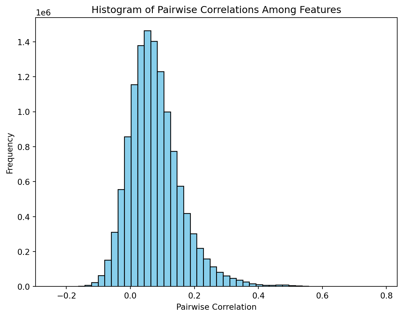
Deep Learning
Defining a Baseline Model
def create_baseline_model(input_dim, hidden_dims):

    """
    Creates a baseline deep feedforward network with the same architecture
    as the graph-embedded model but without domain-specific graph information.

    Architecture:
      - Input layer of dimension 'input_dim'.
      - First hidden layer: Fully connected mapping from input to an output
        with the same dimension (i.e. input_dim), with ReLU activation.
      - Additional Dense hidden layers as specified in hidden_dims.
      - Final output layer with a single neuron for binary classification.

    Args:
      input_dim (int): Number of input features.
      hidden_dims (list of int): List of hidden layer sizes after the first layer.

    Returns:
      model (tf.keras.Model): The baseline Keras model.
    """

    inputs = keras.Input(shape=(input_dim,))

    # First hidden layer: fully connected (without graph-based filtering)
    x = layers.Dense(input_dim, activation="relu", name="baseline_fc1")(inputs)

    # Additional hidden layers
    for i, hdim in enumerate(hidden_dims):
        x = layers.Dense(hdim, activation="relu", name=f"baseline_fc{i+2}")(x)

    # Final output layer (for binary classification)
    outputs = layers.Dense(1, activation="sigmoid", name="output")(x)

    model = keras.Model(inputs=inputs, outputs=outputs)
    return model
Defining a Graph-Embedded Neural Network Model Based on Kong & Yu (2018)
# Custom graph-embedded Dense layer (for reference)

class GraphEmbeddedDense(layers.Layer):
    def __init__(self, units, mask, use_bias=True, **kwargs):

        """
        Custom Dense layer that embeds a feature graph.

        Args:
            units (int): Number of output units (typically equals the input dimension).
            mask (np.array or tf.Tensor): Adjacency matrix of shape (input_dim, units).
            use_bias (bool): Whether to include a bias term.
        """

        super(GraphEmbeddedDense, self).__init__(**kwargs)
        self.units = units
        self.mask = tf.constant(mask, dtype=tf.float32)
        self.use_bias = use_bias

    def build(self, input_shape):
        input_dim = int(input_shape[-1])
        self.kernel = self.add_weight(
            shape=(input_dim, self.units),
            initializer=tf.keras.initializers.HeUniform(),
            trainable=True,
            name="kernel"
        )
        if self.use_bias:
            self.bias = self.add_weight(
                shape=(self.units,),
                initializer="zeros",
                trainable=True,
                name="bias"
            )
        else:
            self.bias = None
        super(GraphEmbeddedDense, self).build(input_shape)

    def call(self, inputs):
        masked_kernel = self.kernel * self.mask
        output = tf.matmul(inputs, masked_kernel)
        if self.use_bias:
            output = output + self.bias
        return output

### Build a Keras model that uses the custom graph-embedded layer.

def create_graph_model(input_dim, hidden_dims, mask):
    inputs = keras.Input(shape=(input_dim,))
    # Graph-embedded layer: name it "graph_layer"
    x = GraphEmbeddedDense(units=input_dim, mask=mask, name="graph_layer")(inputs)
    x = layers.ReLU()(x)
    # First fully connected layer, name it "fc1"
    x = layers.Dense(hidden_dims[0], activation="relu", name="fc1")(x)
    # Additional Dense layers (if any)
    for hdim in hidden_dims[1:]:
        x = layers.Dense(hdim, activation="relu")(x)
    # Final output layer for binary classification
    outputs = layers.Dense(1, activation="sigmoid")(x)
    model = keras.Model(inputs=inputs, outputs=outputs)

    return model

def evaluate_feature_importance_keras(model):

    """
    Evaluate feature importance using the GCW method from Kong & Yu (2018).

    Assumptions:
      - The graph-embedded layer is named "graph_layer". It has attributes:
            • kernel: trainable weight matrix of shape (p, p)
            • mask: fixed binary tensor (adjacency matrix) of shape (p, p)
      - The first Dense layer following the graph layer is named "fc1"
        and has kernel shape (p, h1), where rows correspond to input features.

    Returns:
        importance: a tensor of shape (p,) with the computed importance scores.
    """

    # Retrieve the graph-embedded layer
    graph_layer = model.get_layer("graph_layer")
    # Retrieve the trainable kernel and the fixed mask
    W_in = graph_layer.kernel  # shape: (p, p)
    mask = graph_layer.mask    # shape: (p, p) assumed to be a tf.Tensor

    # Compute the effective weight matrix (only allowed connections)
    effective_W = W_in * mask  # element-wise multiplication

    # For each feature j, sum the absolute weights from the graph layer.
    # Since Keras Dense layers perform: output = x @ kernel, the j-th column
    # corresponds to contributions from feature j.
    graph_contrib = tf.reduce_sum(tf.abs(effective_W), axis=0)  # shape: (p,)

    # Retrieve the first Dense layer after the graph layer (named "fc1")
    fc1 = model.get_layer("fc1")
    # For a Dense layer, kernel shape is (input_dim, units); rows correspond to input features.
    W_fc1 = fc1.kernel  # shape: (p, h1)
    fc1_contrib = tf.reduce_sum(tf.abs(W_fc1), axis=1)  # sum over units → shape: (p,)

    # Compute the degree of each feature from the mask (sum over each column)
    degree = tf.reduce_sum(mask, axis=0)  # shape: (p,)
    eps = 1e-8  # to avoid division by zero
    c = 50
    gamma = tf.minimum(tf.ones_like(degree), c / (degree + eps))

    # Combine the contributions with the penalty factor
    importance = gamma * graph_contrib + fc1_contrib
    return importance
Runs
Creating the Training, Validation, and Test Datasets
# Parameters
n = 400      # number of samples
p = 5000     # number of features
p0 = 40      # number of true predictors

# Generate the synthetic data
X, y, true_idx, R, G, b, b0, prob = generate_synthetic_data(n=n, p=p, p0=p0, random_seed=0)

A = nx.adjacency_matrix(G).todense()
# Split the data: 80% train, 10% validation, 10% test.
X_train, X_temp, y_train, y_temp = train_test_split(X, y, stratify=y, test_size=0.2, random_state=0)
## Scaling
scaler = StandardScaler()
X_train = scaler.fit_transform(X_train)
X_temp = scaler.transform(X_temp)
X_val, X_test, y_val, y_test = train_test_split(X_temp, y_temp, stratify=y_temp, test_size=0.5, random_state=0)
keras.utils.set_random_seed(0)Create the Baseline Model
input_dim = X_train.shape[1]  # e.g., 500 features in synthetic data.
hidden_dims = [64, 16]
baseline_model = create_baseline_model(input_dim=input_dim, hidden_dims=hidden_dims)
baseline_model.compile(optimizer='adam', loss='binary_crossentropy', metrics=['accuracy'])
baseline_model.summary()
Model: "functional_1"
┏━━━━━━━━━━━━━━━━━━━━━━━━━━━━━━━━━┳━━━━━━━━━━━━━━━━━━━━━━━━┳━━━━━━━━━━━━━━━┓
┃ Layer (type)                    ┃ Output Shape           ┃       Param # ┃
┡━━━━━━━━━━━━━━━━━━━━━━━━━━━━━━━━━╇━━━━━━━━━━━━━━━━━━━━━━━━╇━━━━━━━━━━━━━━━┩
│ input_layer_1 (InputLayer)      │ (None, 5000)           │             0 │
├─────────────────────────────────┼────────────────────────┼───────────────┤
│ baseline_fc1 (Dense)            │ (None, 5000)           │    25,005,000 │
├─────────────────────────────────┼────────────────────────┼───────────────┤
│ baseline_fc2 (Dense)            │ (None, 64)             │       320,064 │
├─────────────────────────────────┼────────────────────────┼───────────────┤
│ baseline_fc3 (Dense)            │ (None, 16)             │         1,040 │
├─────────────────────────────────┼────────────────────────┼───────────────┤
│ output (Dense)                  │ (None, 1)              │            17 │
└─────────────────────────────────┴────────────────────────┴───────────────┘
Total params: 25,326,121 (96.61 MB)
Trainable params: 25,326,121 (96.61 MB)
Non-trainable params: 0 (0.00 B)
Train and Visualize Training/Validation Loss
# Define callbacks for early stopping.
callbacks = [
keras.callbacks.EarlyStopping(monitor='val_loss', patience=10, restore_best_weights=True)
]
# Train the baseline model.
history_baseline = baseline_model.fit(X_train, y_train,
validation_data=(X_val, y_val),
epochs=100, batch_size=32, callbacks=callbacks)
# Plot training and validation loss.
plt.figure(figsize=(12, 5))
plt.subplot(1, 2, 1)
plt.plot(history_baseline.history['loss'], label='Baseline Train Loss')
plt.plot(history_baseline.history['val_loss'], label='Baseline Val Loss')
plt.title("Baseline Loss")
plt.xlabel("Epoch")
plt.ylabel("Loss")
plt.legend()
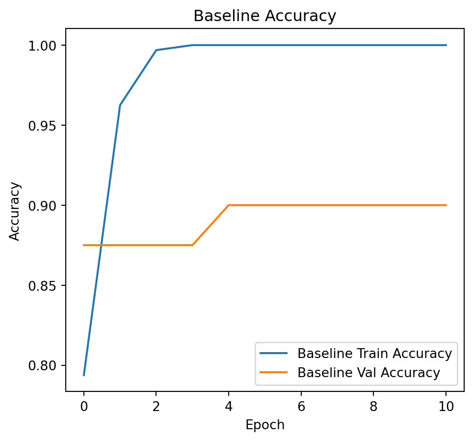
# Plot training and validation loss.
plt.figure(figsize=(12, 5))
plt.subplot(1, 2, 1)
plt.plot(history_baseline.history['accuracy'], label='Baseline Train Accuracy')
plt.plot(history_baseline.history['val_accuracy'], label='Baseline Val Accuracy')
plt.title("Baseline Accuracy")
plt.xlabel("Epoch")
plt.ylabel("Accuracy")
plt.legend()Epoch 1/100
1/10 ━━━━━━━━━━━━━━━━━━━━ 3s 410ms/step - accuracy: 0.6250 - loss: 0.6584 3/10 ━━━━━━━━━━━━━━━━━━━━ 0s 36ms/step - accuracy: 0.6997 - loss: 0.6159 5/10 ━━━━━━━━━━━━━━━━━━━━ 0s 36ms/step - accuracy: 0.7232 - loss: 0.6330 7/10 ━━━━━━━━━━━━━━━━━━━━ 0s 36ms/step - accuracy: 0.7459 - loss: 0.6357 9/10 ━━━━━━━━━━━━━━━━━━━━ 0s 36ms/step - accuracy: 0.7575 - loss: 0.634910/10 ━━━━━━━━━━━━━━━━━━━━ 1s 49ms/step - accuracy: 0.7641 - loss: 0.6366 - val_accuracy: 0.8750 - val_loss: 0.2948
Epoch 2/100
1/10 ━━━━━━━━━━━━━━━━━━━━ 0s 52ms/step - accuracy: 0.9375 - loss: 0.1156 3/10 ━━━━━━━━━━━━━━━━━━━━ 0s 36ms/step - accuracy: 0.9323 - loss: 0.1502 5/10 ━━━━━━━━━━━━━━━━━━━━ 0s 36ms/step - accuracy: 0.9413 - loss: 0.1410 7/10 ━━━━━━━━━━━━━━━━━━━━ 0s 35ms/step - accuracy: 0.9436 - loss: 0.1383 9/10 ━━━━━━━━━━━━━━━━━━━━ 0s 35ms/step - accuracy: 0.9463 - loss: 0.133010/10 ━━━━━━━━━━━━━━━━━━━━ 0s 39ms/step - accuracy: 0.9492 - loss: 0.1269 - val_accuracy: 0.8750 - val_loss: 0.3842
Epoch 3/100
1/10 ━━━━━━━━━━━━━━━━━━━━ 0s 44ms/step - accuracy: 1.0000 - loss: 0.0156 3/10 ━━━━━━━━━━━━━━━━━━━━ 0s 35ms/step - accuracy: 1.0000 - loss: 0.0139 5/10 ━━━━━━━━━━━━━━━━━━━━ 0s 35ms/step - accuracy: 1.0000 - loss: 0.0138 7/10 ━━━━━━━━━━━━━━━━━━━━ 0s 35ms/step - accuracy: 0.9986 - loss: 0.0144 9/10 ━━━━━━━━━━━━━━━━━━━━ 0s 35ms/step - accuracy: 0.9981 - loss: 0.014510/10 ━━━━━━━━━━━━━━━━━━━━ 0s 37ms/step - accuracy: 0.9980 - loss: 0.014510/10 ━━━━━━━━━━━━━━━━━━━━ 0s 41ms/step - accuracy: 0.9979 - loss: 0.0145 - val_accuracy: 0.8750 - val_loss: 0.4570
Epoch 4/100
1/10 ━━━━━━━━━━━━━━━━━━━━ 0s 43ms/step - accuracy: 1.0000 - loss: 1.4341e-04 3/10 ━━━━━━━━━━━━━━━━━━━━ 0s 35ms/step - accuracy: 1.0000 - loss: 5.2759e-04 5/10 ━━━━━━━━━━━━━━━━━━━━ 0s 35ms/step - accuracy: 1.0000 - loss: 7.4482e-04 7/10 ━━━━━━━━━━━━━━━━━━━━ 0s 35ms/step - accuracy: 1.0000 - loss: 9.7139e-04 9/10 ━━━━━━━━━━━━━━━━━━━━ 0s 35ms/step - accuracy: 1.0000 - loss: 0.0011 10/10 ━━━━━━━━━━━━━━━━━━━━ 0s 39ms/step - accuracy: 1.0000 - loss: 0.0012 - val_accuracy: 0.8750 - val_loss: 0.4990
Epoch 5/100
1/10 ━━━━━━━━━━━━━━━━━━━━ 0s 43ms/step - accuracy: 1.0000 - loss: 9.3608e-05 3/10 ━━━━━━━━━━━━━━━━━━━━ 0s 36ms/step - accuracy: 1.0000 - loss: 3.2221e-04 5/10 ━━━━━━━━━━━━━━━━━━━━ 0s 40ms/step - accuracy: 1.0000 - loss: 4.5092e-04 7/10 ━━━━━━━━━━━━━━━━━━━━ 0s 38ms/step - accuracy: 1.0000 - loss: 5.3923e-04 9/10 ━━━━━━━━━━━━━━━━━━━━ 0s 38ms/step - accuracy: 1.0000 - loss: 6.1852e-0410/10 ━━━━━━━━━━━━━━━━━━━━ 0s 41ms/step - accuracy: 1.0000 - loss: 6.5996e-04 - val_accuracy: 0.9000 - val_loss: 0.5234
Epoch 6/100
1/10 ━━━━━━━━━━━━━━━━━━━━ 0s 45ms/step - accuracy: 1.0000 - loss: 7.4949e-05 3/10 ━━━━━━━━━━━━━━━━━━━━ 0s 35ms/step - accuracy: 1.0000 - loss: 2.2841e-04 5/10 ━━━━━━━━━━━━━━━━━━━━ 0s 35ms/step - accuracy: 1.0000 - loss: 3.1009e-04 7/10 ━━━━━━━━━━━━━━━━━━━━ 0s 35ms/step - accuracy: 1.0000 - loss: 3.6075e-04 9/10 ━━━━━━━━━━━━━━━━━━━━ 0s 36ms/step - accuracy: 1.0000 - loss: 4.1217e-0410/10 ━━━━━━━━━━━━━━━━━━━━ 0s 40ms/step - accuracy: 1.0000 - loss: 4.4008e-04 - val_accuracy: 0.9000 - val_loss: 0.5367
Epoch 7/100
1/10 ━━━━━━━━━━━━━━━━━━━━ 0s 44ms/step - accuracy: 1.0000 - loss: 6.0929e-05 3/10 ━━━━━━━━━━━━━━━━━━━━ 0s 36ms/step - accuracy: 1.0000 - loss: 1.7496e-04 5/10 ━━━━━━━━━━━━━━━━━━━━ 0s 36ms/step - accuracy: 1.0000 - loss: 2.3425e-04 7/10 ━━━━━━━━━━━━━━━━━━━━ 0s 36ms/step - accuracy: 1.0000 - loss: 2.6941e-04 9/10 ━━━━━━━━━━━━━━━━━━━━ 0s 35ms/step - accuracy: 1.0000 - loss: 3.0838e-0410/10 ━━━━━━━━━━━━━━━━━━━━ 0s 39ms/step - accuracy: 1.0000 - loss: 3.3020e-04 - val_accuracy: 0.9000 - val_loss: 0.5448
Epoch 8/100
1/10 ━━━━━━━━━━━━━━━━━━━━ 0s 44ms/step - accuracy: 1.0000 - loss: 5.0238e-05 3/10 ━━━━━━━━━━━━━━━━━━━━ 0s 36ms/step - accuracy: 1.0000 - loss: 1.4175e-04 5/10 ━━━━━━━━━━━━━━━━━━━━ 0s 36ms/step - accuracy: 1.0000 - loss: 1.8926e-04 7/10 ━━━━━━━━━━━━━━━━━━━━ 0s 36ms/step - accuracy: 1.0000 - loss: 2.1658e-04 9/10 ━━━━━━━━━━━━━━━━━━━━ 0s 36ms/step - accuracy: 1.0000 - loss: 2.4840e-0410/10 ━━━━━━━━━━━━━━━━━━━━ 0s 40ms/step - accuracy: 1.0000 - loss: 2.6659e-04 - val_accuracy: 0.9000 - val_loss: 0.5504
Epoch 9/100
1/10 ━━━━━━━━━━━━━━━━━━━━ 0s 42ms/step - accuracy: 1.0000 - loss: 4.2559e-05 3/10 ━━━━━━━━━━━━━━━━━━━━ 0s 35ms/step - accuracy: 1.0000 - loss: 1.1920e-04 5/10 ━━━━━━━━━━━━━━━━━━━━ 0s 35ms/step - accuracy: 1.0000 - loss: 1.5944e-04 7/10 ━━━━━━━━━━━━━━━━━━━━ 0s 35ms/step - accuracy: 1.0000 - loss: 1.8210e-04 9/10 ━━━━━━━━━━━━━━━━━━━━ 0s 35ms/step - accuracy: 1.0000 - loss: 2.0921e-0410/10 ━━━━━━━━━━━━━━━━━━━━ 0s 39ms/step - accuracy: 1.0000 - loss: 2.2492e-04 - val_accuracy: 0.9000 - val_loss: 0.5549
Epoch 10/100
1/10 ━━━━━━━━━━━━━━━━━━━━ 0s 44ms/step - accuracy: 1.0000 - loss: 3.6963e-05 3/10 ━━━━━━━━━━━━━━━━━━━━ 0s 35ms/step - accuracy: 1.0000 - loss: 1.0288e-04 5/10 ━━━━━━━━━━━━━━━━━━━━ 0s 35ms/step - accuracy: 1.0000 - loss: 1.3799e-04 7/10 ━━━━━━━━━━━━━━━━━━━━ 0s 35ms/step - accuracy: 1.0000 - loss: 1.5764e-04 9/10 ━━━━━━━━━━━━━━━━━━━━ 0s 36ms/step - accuracy: 1.0000 - loss: 1.8145e-0410/10 ━━━━━━━━━━━━━━━━━━━━ 0s 40ms/step - accuracy: 1.0000 - loss: 1.9536e-04 - val_accuracy: 0.9000 - val_loss: 0.5587
Epoch 11/100
1/10 ━━━━━━━━━━━━━━━━━━━━ 0s 45ms/step - accuracy: 1.0000 - loss: 3.2823e-05 3/10 ━━━━━━━━━━━━━━━━━━━━ 0s 35ms/step - accuracy: 1.0000 - loss: 9.0570e-05 5/10 ━━━━━━━━━━━━━━━━━━━━ 0s 35ms/step - accuracy: 1.0000 - loss: 1.2171e-04 7/10 ━━━━━━━━━━━━━━━━━━━━ 0s 35ms/step - accuracy: 1.0000 - loss: 1.3897e-04 9/10 ━━━━━━━━━━━━━━━━━━━━ 0s 35ms/step - accuracy: 1.0000 - loss: 1.6007e-0410/10 ━━━━━━━━━━━━━━━━━━━━ 0s 39ms/step - accuracy: 1.0000 - loss: 1.7248e-04 - val_accuracy: 0.9000 - val_loss: 0.5622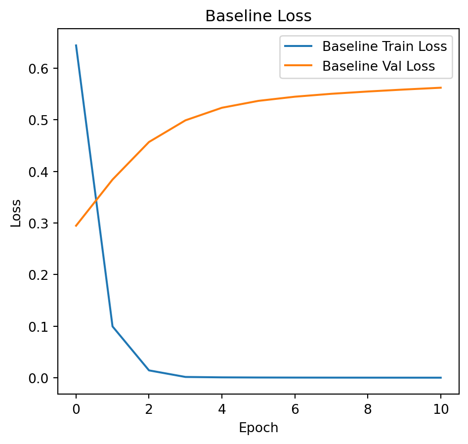
Create the Graph-Embedded Model
# Now, use A as the mask for GraphEmbeddedNetwork:
graph_model = create_graph_model(input_dim, hidden_dims, A)
graph_model.compile(optimizer='adam', loss='binary_crossentropy', metrics=['accuracy'])
graph_model.summary()
Model: "functional_2"
┏━━━━━━━━━━━━━━━━━━━━━━━━━━━━━━━━━┳━━━━━━━━━━━━━━━━━━━━━━━━┳━━━━━━━━━━━━━━━┓
┃ Layer (type)                    ┃ Output Shape           ┃       Param # ┃
┡━━━━━━━━━━━━━━━━━━━━━━━━━━━━━━━━━╇━━━━━━━━━━━━━━━━━━━━━━━━╇━━━━━━━━━━━━━━━┩
│ input_layer_2 (InputLayer)      │ (None, 5000)           │             0 │
├─────────────────────────────────┼────────────────────────┼───────────────┤
│ graph_layer                     │ (None, 5000)           │    25,005,000 │
│ (GraphEmbeddedDense)            │                        │               │
├─────────────────────────────────┼────────────────────────┼───────────────┤
│ re_lu (ReLU)                    │ (None, 5000)           │             0 │
├─────────────────────────────────┼────────────────────────┼───────────────┤
│ fc1 (Dense)                     │ (None, 64)             │       320,064 │
├─────────────────────────────────┼────────────────────────┼───────────────┤
│ dense (Dense)                   │ (None, 16)             │         1,040 │
├─────────────────────────────────┼────────────────────────┼───────────────┤
│ dense_1 (Dense)                 │ (None, 1)              │            17 │
└─────────────────────────────────┴────────────────────────┴───────────────┘
Total params: 25,326,121 (96.61 MB)
Trainable params: 25,326,121 (96.61 MB)
Non-trainable params: 0 (0.00 B)
Train and Visualize Training/Validation Loss
# Train the graph-embedded model.
history_graph = graph_model.fit(X_train, y_train,
validation_data=(X_val, y_val),
epochs=100, batch_size=32, callbacks=callbacks)
plt.subplot(1, 2, 2)
plt.plot(history_graph.history['loss'], label='GraphModel Train Loss')
plt.plot(history_graph.history['val_loss'], label='GraphModel Val Loss')
plt.title("Graph-Embedded Model Loss")
plt.xlabel("Epoch")
plt.ylabel("Loss")
plt.legend()
plt.show()
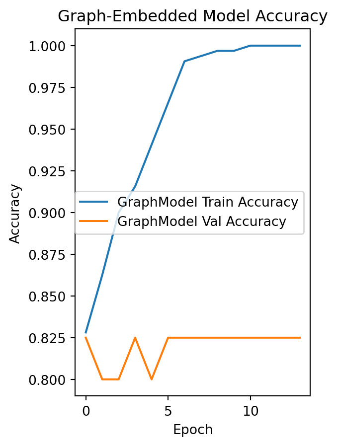
plt.subplot(1, 2, 2)
plt.plot(history_graph.history['accuracy'], label='GraphModel Train Accuracy')
plt.plot(history_graph.history['val_accuracy'], label='GraphModel Val Accuracy')
plt.title("Graph-Embedded Model Accuracy")
plt.xlabel("Epoch")
plt.ylabel("Accuracy")
plt.legend()
plt.show()
importance_scores = evaluate_feature_importance_keras(graph_model)
print("Feature importance scores (shape {}):".format(importance_scores.shape))
print(importance_scores.numpy())Epoch 1/100
1/10 ━━━━━━━━━━━━━━━━━━━━ 3s 422ms/step - accuracy: 0.4375 - loss: 0.6943 3/10 ━━━━━━━━━━━━━━━━━━━━ 0s 40ms/step - accuracy: 0.6111 - loss: 0.6873 5/10 ━━━━━━━━━━━━━━━━━━━━ 0s 40ms/step - accuracy: 0.6717 - loss: 0.6777 7/10 ━━━━━━━━━━━━━━━━━━━━ 0s 40ms/step - accuracy: 0.7083 - loss: 0.6674 9/10 ━━━━━━━━━━━━━━━━━━━━ 0s 40ms/step - accuracy: 0.7322 - loss: 0.656510/10 ━━━━━━━━━━━━━━━━━━━━ 1s 54ms/step - accuracy: 0.7497 - loss: 0.6454 - val_accuracy: 0.8250 - val_loss: 0.4912
Epoch 2/100
1/10 ━━━━━━━━━━━━━━━━━━━━ 0s 56ms/step - accuracy: 0.8750 - loss: 0.4832 3/10 ━━━━━━━━━━━━━━━━━━━━ 0s 40ms/step - accuracy: 0.8681 - loss: 0.4581 5/10 ━━━━━━━━━━━━━━━━━━━━ 0s 40ms/step - accuracy: 0.8596 - loss: 0.4453 7/10 ━━━━━━━━━━━━━━━━━━━━ 0s 40ms/step - accuracy: 0.8605 - loss: 0.4324 9/10 ━━━━━━━━━━━━━━━━━━━━ 0s 40ms/step - accuracy: 0.8613 - loss: 0.422010/10 ━━━━━━━━━━━━━━━━━━━━ 0s 46ms/step - accuracy: 0.8615 - loss: 0.4133 - val_accuracy: 0.8000 - val_loss: 0.3476
Epoch 3/100
1/10 ━━━━━━━━━━━━━━━━━━━━ 0s 50ms/step - accuracy: 0.8438 - loss: 0.3099 3/10 ━━━━━━━━━━━━━━━━━━━━ 0s 41ms/step - accuracy: 0.8681 - loss: 0.2919 5/10 ━━━━━━━━━━━━━━━━━━━━ 0s 40ms/step - accuracy: 0.8721 - loss: 0.2908 7/10 ━━━━━━━━━━━━━━━━━━━━ 0s 40ms/step - accuracy: 0.8770 - loss: 0.2873 9/10 ━━━━━━━━━━━━━━━━━━━━ 0s 40ms/step - accuracy: 0.8814 - loss: 0.283010/10 ━━━━━━━━━━━━━━━━━━━━ 0s 46ms/step - accuracy: 0.8848 - loss: 0.2795 - val_accuracy: 0.8000 - val_loss: 0.3347
Epoch 4/100
1/10 ━━━━━━━━━━━━━━━━━━━━ 0s 50ms/step - accuracy: 0.8750 - loss: 0.2589 3/10 ━━━━━━━━━━━━━━━━━━━━ 0s 39ms/step - accuracy: 0.8872 - loss: 0.2378 5/10 ━━━━━━━━━━━━━━━━━━━━ 0s 40ms/step - accuracy: 0.8948 - loss: 0.2352 7/10 ━━━━━━━━━━━━━━━━━━━━ 0s 40ms/step - accuracy: 0.8987 - loss: 0.2324 9/10 ━━━━━━━━━━━━━━━━━━━━ 0s 40ms/step - accuracy: 0.9020 - loss: 0.228510/10 ━━━━━━━━━━━━━━━━━━━━ 0s 46ms/step - accuracy: 0.9045 - loss: 0.2251 - val_accuracy: 0.8250 - val_loss: 0.3311
Epoch 5/100
1/10 ━━━━━━━━━━━━━━━━━━━━ 0s 49ms/step - accuracy: 0.9375 - loss: 0.2122 3/10 ━━━━━━━━━━━━━━━━━━━━ 0s 40ms/step - accuracy: 0.9427 - loss: 0.1899 5/10 ━━━━━━━━━━━━━━━━━━━━ 0s 40ms/step - accuracy: 0.9447 - loss: 0.1876 7/10 ━━━━━━━━━━━━━━━━━━━━ 0s 40ms/step - accuracy: 0.9440 - loss: 0.1846 9/10 ━━━━━━━━━━━━━━━━━━━━ 0s 40ms/step - accuracy: 0.9438 - loss: 0.181310/10 ━━━━━━━━━━━━━━━━━━━━ 0s 44ms/step - accuracy: 0.9432 - loss: 0.1785 - val_accuracy: 0.8000 - val_loss: 0.3316
Epoch 6/100
1/10 ━━━━━━━━━━━━━━━━━━━━ 0s 48ms/step - accuracy: 0.9688 - loss: 0.1502 3/10 ━━━━━━━━━━━━━━━━━━━━ 0s 40ms/step - accuracy: 0.9618 - loss: 0.1354 5/10 ━━━━━━━━━━━━━━━━━━━━ 0s 40ms/step - accuracy: 0.9602 - loss: 0.1350 7/10 ━━━━━━━━━━━━━━━━━━━━ 0s 40ms/step - accuracy: 0.9585 - loss: 0.1327 9/10 ━━━━━━━━━━━━━━━━━━━━ 0s 40ms/step - accuracy: 0.9591 - loss: 0.130510/10 ━━━━━━━━━━━━━━━━━━━━ 0s 45ms/step - accuracy: 0.9603 - loss: 0.1287 - val_accuracy: 0.8250 - val_loss: 0.3326
Epoch 7/100
1/10 ━━━━━━━━━━━━━━━━━━━━ 0s 48ms/step - accuracy: 0.9688 - loss: 0.0911 3/10 ━━━━━━━━━━━━━━━━━━━━ 0s 40ms/step - accuracy: 0.9809 - loss: 0.0844 5/10 ━━━━━━━━━━━━━━━━━━━━ 0s 40ms/step - accuracy: 0.9829 - loss: 0.0851 7/10 ━━━━━━━━━━━━━━━━━━━━ 0s 40ms/step - accuracy: 0.9850 - loss: 0.0836 9/10 ━━━━━━━━━━━━━━━━━━━━ 0s 40ms/step - accuracy: 0.9863 - loss: 0.082810/10 ━━━━━━━━━━━━━━━━━━━━ 0s 45ms/step - accuracy: 0.9871 - loss: 0.0823 - val_accuracy: 0.8250 - val_loss: 0.3400
Epoch 8/100
1/10 ━━━━━━━━━━━━━━━━━━━━ 0s 49ms/step - accuracy: 1.0000 - loss: 0.0505 3/10 ━━━━━━━━━━━━━━━━━━━━ 0s 39ms/step - accuracy: 1.0000 - loss: 0.0482 5/10 ━━━━━━━━━━━━━━━━━━━━ 0s 40ms/step - accuracy: 0.9972 - loss: 0.0481 7/10 ━━━━━━━━━━━━━━━━━━━━ 0s 40ms/step - accuracy: 0.9966 - loss: 0.0471 9/10 ━━━━━━━━━━━━━━━━━━━━ 0s 40ms/step - accuracy: 0.9962 - loss: 0.047310/10 ━━━━━━━━━━━━━━━━━━━━ 0s 45ms/step - accuracy: 0.9957 - loss: 0.0477 - val_accuracy: 0.8250 - val_loss: 0.3513
Epoch 9/100
1/10 ━━━━━━━━━━━━━━━━━━━━ 0s 49ms/step - accuracy: 1.0000 - loss: 0.0293 3/10 ━━━━━━━━━━━━━━━━━━━━ 0s 40ms/step - accuracy: 1.0000 - loss: 0.0278 5/10 ━━━━━━━━━━━━━━━━━━━━ 0s 40ms/step - accuracy: 1.0000 - loss: 0.0271 7/10 ━━━━━━━━━━━━━━━━━━━━ 0s 40ms/step - accuracy: 1.0000 - loss: 0.0265 9/10 ━━━━━━━━━━━━━━━━━━━━ 0s 40ms/step - accuracy: 0.9996 - loss: 0.027010/10 ━━━━━━━━━━━━━━━━━━━━ 0s 44ms/step - accuracy: 0.9991 - loss: 0.0277 - val_accuracy: 0.8250 - val_loss: 0.3674
Epoch 10/100
1/10 ━━━━━━━━━━━━━━━━━━━━ 0s 49ms/step - accuracy: 1.0000 - loss: 0.0182 3/10 ━━━━━━━━━━━━━━━━━━━━ 0s 40ms/step - accuracy: 1.0000 - loss: 0.0169 5/10 ━━━━━━━━━━━━━━━━━━━━ 0s 40ms/step - accuracy: 1.0000 - loss: 0.0165 7/10 ━━━━━━━━━━━━━━━━━━━━ 0s 40ms/step - accuracy: 1.0000 - loss: 0.0161 9/10 ━━━━━━━━━━━━━━━━━━━━ 0s 40ms/step - accuracy: 0.9996 - loss: 0.016510/10 ━━━━━━━━━━━━━━━━━━━━ 0s 44ms/step - accuracy: 0.9991 - loss: 0.0170 - val_accuracy: 0.8250 - val_loss: 0.3861
Epoch 11/100
1/10 ━━━━━━━━━━━━━━━━━━━━ 0s 49ms/step - accuracy: 1.0000 - loss: 0.0117 3/10 ━━━━━━━━━━━━━━━━━━━━ 0s 40ms/step - accuracy: 1.0000 - loss: 0.0110 5/10 ━━━━━━━━━━━━━━━━━━━━ 0s 40ms/step - accuracy: 1.0000 - loss: 0.0108 7/10 ━━━━━━━━━━━━━━━━━━━━ 0s 40ms/step - accuracy: 1.0000 - loss: 0.0106 9/10 ━━━━━━━━━━━━━━━━━━━━ 0s 40ms/step - accuracy: 1.0000 - loss: 0.010710/10 ━━━━━━━━━━━━━━━━━━━━ 0s 45ms/step - accuracy: 1.0000 - loss: 0.0107 - val_accuracy: 0.8250 - val_loss: 0.4065
Epoch 12/100
1/10 ━━━━━━━━━━━━━━━━━━━━ 0s 48ms/step - accuracy: 1.0000 - loss: 0.0079 3/10 ━━━━━━━━━━━━━━━━━━━━ 0s 39ms/step - accuracy: 1.0000 - loss: 0.0075 5/10 ━━━━━━━━━━━━━━━━━━━━ 0s 40ms/step - accuracy: 1.0000 - loss: 0.0074 7/10 ━━━━━━━━━━━━━━━━━━━━ 0s 39ms/step - accuracy: 1.0000 - loss: 0.0073 9/10 ━━━━━━━━━━━━━━━━━━━━ 0s 40ms/step - accuracy: 1.0000 - loss: 0.007310/10 ━━━━━━━━━━━━━━━━━━━━ 0s 45ms/step - accuracy: 1.0000 - loss: 0.0072 - val_accuracy: 0.8250 - val_loss: 0.4293
Epoch 13/100
1/10 ━━━━━━━━━━━━━━━━━━━━ 0s 48ms/step - accuracy: 1.0000 - loss: 0.0056 3/10 ━━━━━━━━━━━━━━━━━━━━ 0s 40ms/step - accuracy: 1.0000 - loss: 0.0054 5/10 ━━━━━━━━━━━━━━━━━━━━ 0s 40ms/step - accuracy: 1.0000 - loss: 0.0053 7/10 ━━━━━━━━━━━━━━━━━━━━ 0s 40ms/step - accuracy: 1.0000 - loss: 0.0052 9/10 ━━━━━━━━━━━━━━━━━━━━ 0s 40ms/step - accuracy: 1.0000 - loss: 0.005210/10 ━━━━━━━━━━━━━━━━━━━━ 0s 45ms/step - accuracy: 1.0000 - loss: 0.0052 - val_accuracy: 0.8250 - val_loss: 0.4457
Epoch 14/100
1/10 ━━━━━━━━━━━━━━━━━━━━ 0s 49ms/step - accuracy: 1.0000 - loss: 0.0043 3/10 ━━━━━━━━━━━━━━━━━━━━ 0s 40ms/step - accuracy: 1.0000 - loss: 0.0041 5/10 ━━━━━━━━━━━━━━━━━━━━ 0s 40ms/step - accuracy: 1.0000 - loss: 0.0040 7/10 ━━━━━━━━━━━━━━━━━━━━ 0s 40ms/step - accuracy: 1.0000 - loss: 0.0040 9/10 ━━━━━━━━━━━━━━━━━━━━ 0s 40ms/step - accuracy: 1.0000 - loss: 0.004010/10 ━━━━━━━━━━━━━━━━━━━━ 0s 45ms/step - accuracy: 1.0000 - loss: 0.0040 - val_accuracy: 0.8250 - val_loss: 0.4607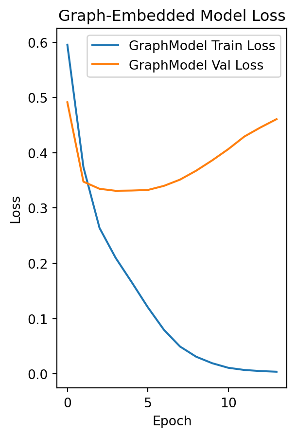
Feature importance scores (shape (5000,)):
[2.9373732 1.7428389 2.3859673 ... 1.2631431 1.1794165 1.4094478]
Evaluate and Compare the Models on the Test Set
# Evaluate the baseline model.
baseline_eval = baseline_model.evaluate(X_test, y_test, verbose=0)
print("Baseline Model")

y_pred = (baseline_model.predict(X_test) > 0.5).astype(int)

print(classification_report(y_test, y_pred))
Baseline Model
1/2 ━━━━━━━━━━━━━━━━━━━━ 0s 28ms/step2/2 ━━━━━━━━━━━━━━━━━━━━ 0s 26ms/step
precision recall f1-score support
0 0.83 0.86 0.84 22
1 0.82 0.78 0.80 18
accuracy 0.82 40
macro avg 0.82 0.82 0.82 40
weighted avg 0.82 0.82 0.82 40
# Evaluate the graph-embedded model.
graph_eval = graph_model.evaluate(X_test, y_test, verbose=0)
print("Graph-Embedded Model:")

y_pred = (graph_model.predict(X_test) > 0.5).astype(int)

print(classification_report(y_test, y_pred))
Graph-Embedded Model:
1/2 ━━━━━━━━━━━━━━━━━━━━ 0s 30ms/step2/2 ━━━━━━━━━━━━━━━━━━━━ 0s 31ms/step
precision recall f1-score support
0 0.87 0.91 0.89 22
1 0.88 0.83 0.86 18
accuracy 0.88 40
macro avg 0.88 0.87 0.87 40
weighted avg 0.88 0.88 0.87 40