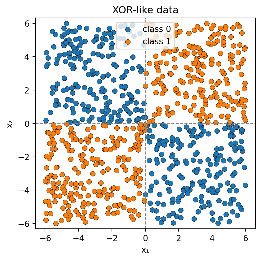
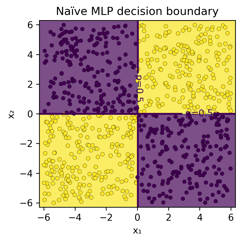
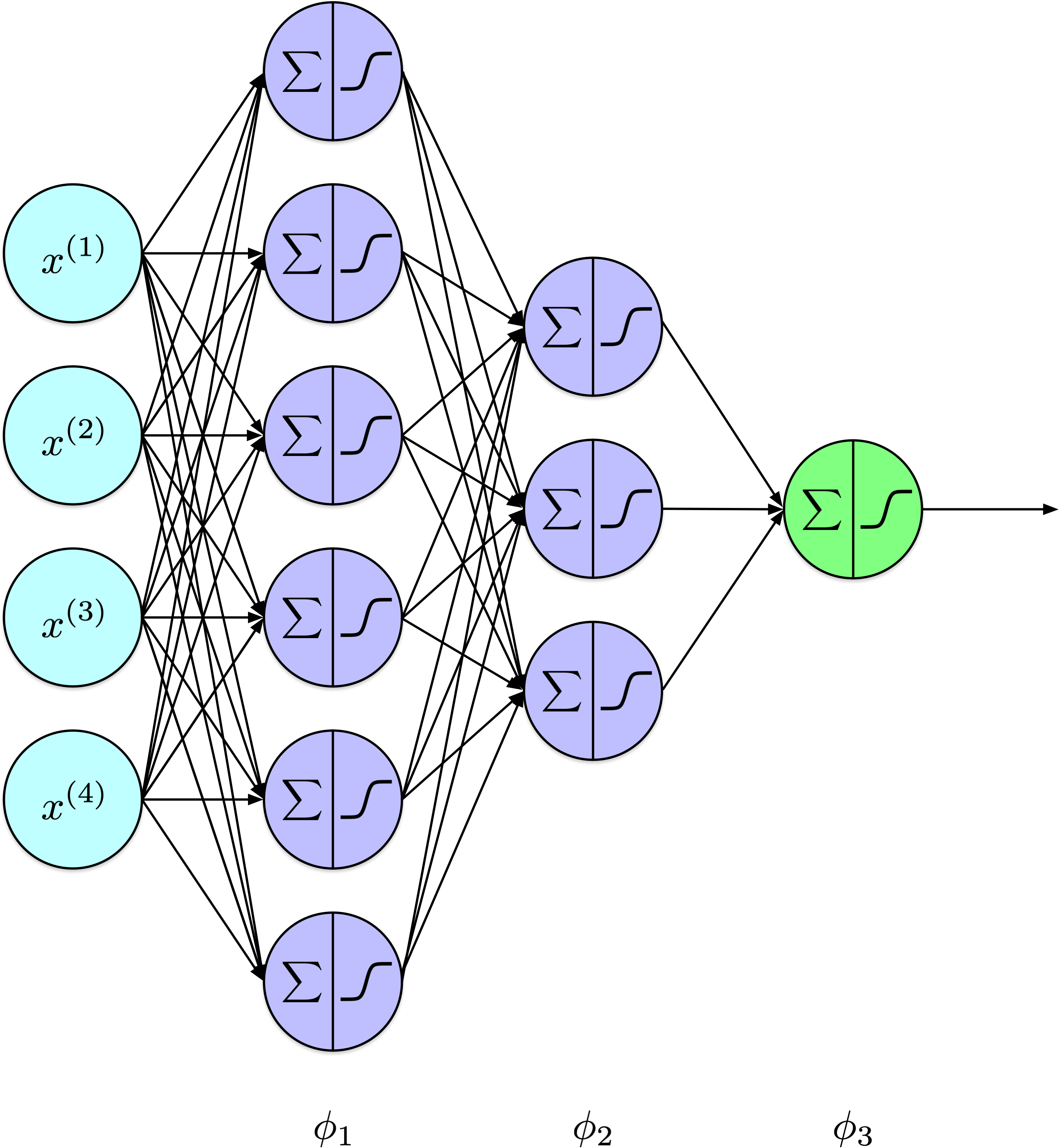
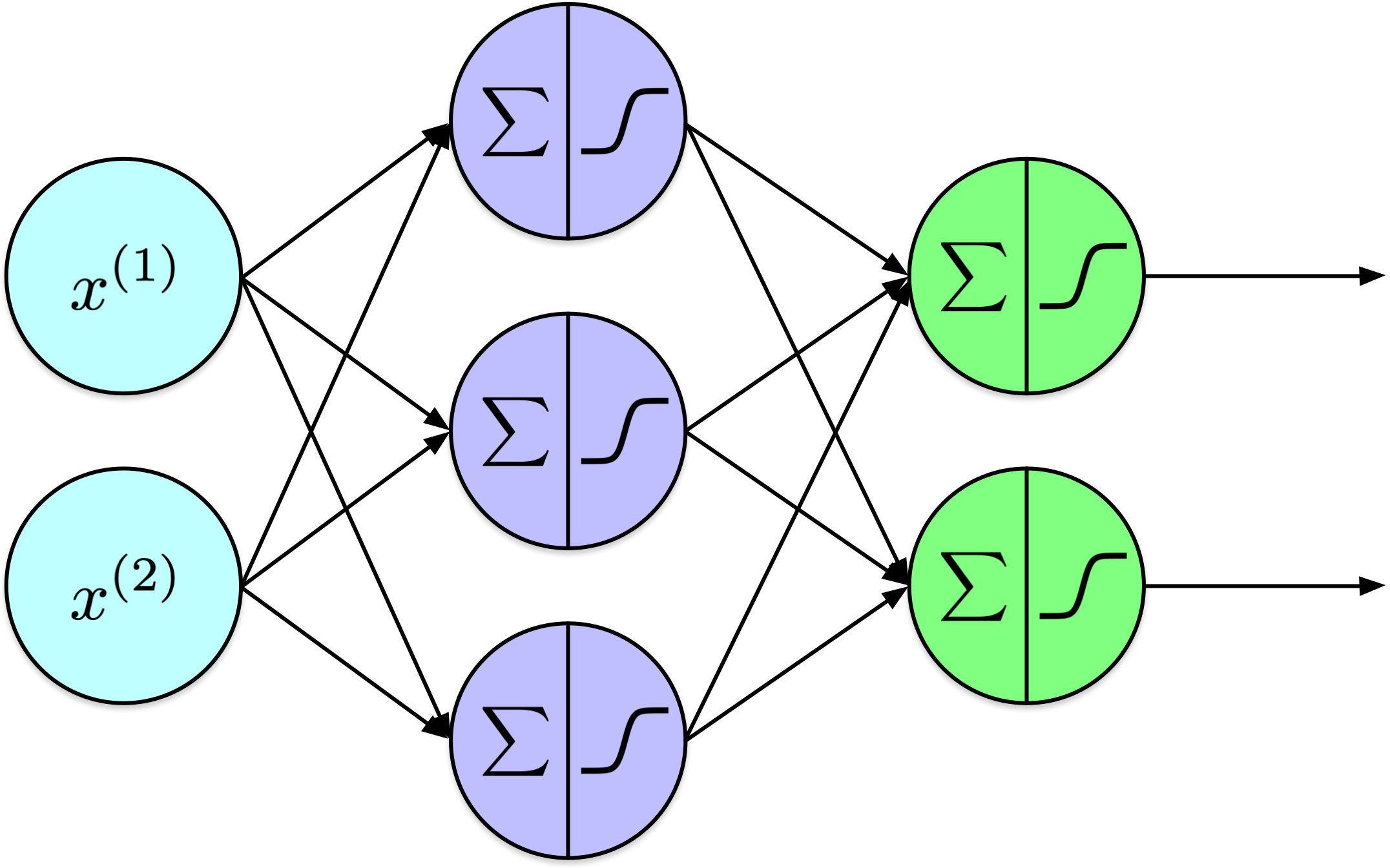
Training Artificial Neural Networks (Part 1)

CSI 4106 - Fall 2025

Marcel Turcotte

Version: Nov 4, 2025 15:11

Preamble

Message of the Day

The text describes a podcast featuring Julian Togelius, an Associate Professor at New York University and co-director of the Game Innovation Lab. Togelius is the author of “Artificial Intelligence and Games,” which has a second edition released in 2025. For those with access to a device on the University of Ottawa’s network, a copy of this book is available for download.

• Artificial Intelligence and Games
  • PDF, EPUB

I have been following Julian Togelius on social media for some time, although I have not yet had the opportunity to read his book.

From Turing’s Chess to Neural Game Engines: AI in Video Games Today by Alex Landa, ODSC, 2025-09-02, a Podcast (1h 8m) featuring Julian Togelius, an Associate Professor at New York University.

Learning objectives

• Explain the architecture and function of feed-forward neural networks (FNNs).
• Identify common activation functions and understand their impact on network performance.
• Introduce a simple but functional implementation of a feed-forward neural networks.

Summary

3Blue1Brown (1/2)

It is highly recommended that you watch this video. While it covers the concepts we have already explored, it presents the material in a manner that is challenging to replicate in a classroom setting.

• Provides a clear explanation of the intuition behind the effectiveness of neural networks, detailing the hierarchy of concepts briefly mentioned in the last lecture. (5m 31s to 8m 38s)
• Offers a compelling rationale for the necessity of a bias term.
• Similarly, elucidates the concept of activation functions and the importance of a squashing function.
• The segment beginning at 13m 26s offers a visual explanation of the linear algebra involved: \(\sigma(W X^T + b)\).

In my opinion, this is an excellent and informative video.

3Blue1Brown (2/2)

We will revisit the concept of gradient descent in our discussion on the backpropagation algorithm. To review this topic, you can watch this video: Gradient descent, how neural networks learn | Deep Learning Chapter 2 (duration: 20 minutes and 33 seconds).

Our discussion will be on backpropagation. Viewing Gradient descent, how neural networks learn might be helpful.

Summary - DL

• Deep learning (DL) is a machine learning technique that can be applied to supervised learning (including regression and classification), unsupervised learning, and reinforcement learning.

• Inspired from the structure and function of biological neural networks found in animals.

• Comprises interconnected neurons (or units) arranged into layers.

Summary - FNN

Neural networks have inputs and outputs.

The network consists of three layers: input, hidden, and output. The input layer contains two nodes, the hidden layer comprises three nodes, and the output layer has two nodes. Additional hidden layers and nodes per layer can be added, which will be discussed later.

It is often useful to include explicit input nodes that do not perform calculations, known as input units or input neurons. These nodes act as placeholders to introduce input features into the network, passing data directly to the next layer without transformation. In the network diagram, these are the light blue nodes on the left. Typically, the number of input units corresponds to the number of features.

Information in this architecture flows unidirectionally—from left to right, moving from input to output. Consequently, it is termed a feed-forward neural network (FNN).

Summary - FNN

Neural networks can have a significantly large number of input nodes, often in the hundreds or thousands, depending on the complexity of the data. Additionally, they may contain numerous hidden layers. For instance, ResNet, which won the ILSVRC 2015 image classification task, features 152 layers. The authors of ResNet have demonstrated results for networks with 100 and even 1000 layers (He et al. 2016). However, the number of output nodes tends to be relatively small. In regression problems, there is typically one output node, while in classification tasks (whether multiclass or multilabel), the number of output nodes corresponds to the number of classes.

Consider a scenario in which one can determine the optimal number of layers and nodes for a neural network. Empirical evidence suggests that such networks excel in performing both classification and regression tasks. Despite the complexity arising from a large number of parameters, which complicates the interpretation of learned patterns, understanding the forward pass, how the network generates predictions from new input data, is relatively straightforward.

Today’s objective is to understand the process of adjusting the network’s weights based on its current output. Specifically, we aim to understand how to utilize the output signal to propagate information backward through the network.

The number of layers and nodes can vary based on the specific requirements.

Summary - units

In the diagram above, it is important to clarify that the inputs and output pertain specifically to this individual unit, rather than to the entire network’s global inputs and output.

The name activation originates from the function’s role in determining whether a neuron should be “activated” or “fired” based on its input.

Historically, the concept was inspired by biological neurons, where a neuron activates and transmits a signal to other neurons if its input exceeds a certain threshold. In artificial neural networks, the activation function serves a similar purpose by introducing non-linearity into the model. This non-linearity is crucial because it enables the network to learn complex patterns and representations in the data.

Introducing a fictitious input \(x^{(0)} = 1\) is a hack that simplifies the expression \(x^T\theta + b\).

Common Activation Functions

# Attribution: https://github.com/ageron/handson-ml3/blob/main/10_neural_nets_with_keras.ipynb

import numpy as np
import matplotlib.pyplot as plt

from scipy.special import expit as sigmoid

def relu(z):
    return np.maximum(0, z)

def derivative(f, z, eps=0.000001):
    return (f(z + eps) - f(z - eps))/(2 * eps)

max_z = 4.5
z = np.linspace(-max_z, max_z, 200)

plt.figure(figsize=(11, 3.1))

plt.subplot(121)
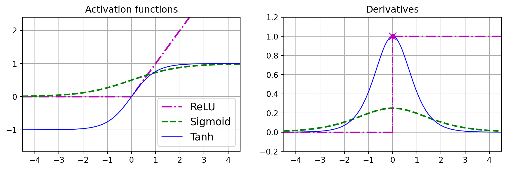
plt.plot(z, relu(z), "m-.", linewidth=2, label="ReLU")
plt.plot(z, sigmoid(z), "g--", linewidth=2, label="Sigmoid")
plt.plot(z, np.tanh(z), "b-", linewidth=1, label="Tanh")
plt.grid(True)
plt.title("Activation functions")
plt.axis([-max_z, max_z, -1.65, 2.4])
plt.gca().set_yticks([-1, 0, 1, 2])
plt.legend(loc="lower right", fontsize=13)

plt.subplot(122)
plt.plot(z, derivative(sigmoid, z), "g--", linewidth=2, label="Sigmoid")
plt.plot(z, derivative(np.tanh, z), "b-", linewidth=1, label="Tanh")
plt.plot([-max_z, 0], [0, 0], "m-.", linewidth=2)
plt.plot([0, max_z], [1, 1], "m-.", linewidth=2)
plt.plot([0, 0], [0, 1], "m-.", linewidth=1.2)
plt.plot(0, 1, "mo", markersize=5)
plt.plot(0, 1, "mx", markersize=10)
plt.grid(True)
plt.title("Derivatives")
plt.axis([-max_z, max_z, -0.2, 1.2])

plt.show()

Consider the following observations:

• The sigmoid function produces outputs within the open interval \((0, 1)\).
• The hyperbolic tangent function (\(\tanh\)) has an image spanning the open interval \((-1, 1)\).
• The Rectified Linear Unit (ReLU) function outputs values in the interval \([0, \infty)\).

Additionally, note:

• The maximum derivative value of the sigmoid function is 0.25.
• The maximum derivative value of the \(\tanh\) function is 1.
• The derivative of the ReLU function is 0 for negative inputs and 1 for positive inputs.

Furthermore:

• A node employing ReLU as its activation function generates outputs within the range \([0, \infty)\). However, its derivative, utilized in gradient descent during backpropagation, is constant, taking values of either 0 or 1.

Géron (2022) – 10_neural_nets_with_keras.ipynb

Universal Approximation

The universal approximation theorem states that a feed-forward neural network with a single hidden layer containing a finite number of neurons can approximate any continuous function on a compact subset of \(\mathbb{R}^n\), given appropriate weights and activation functions.

The Universal Approximation Theorem (UAT) is a powerful theoretical assurance: in principle, a sufficiently wide single-hidden-layer network can approximate any continuous function. But it is not a practical prescription. In real problems, a deep architecture often achieves the same approximation accuracy with far fewer parameters and in a way that is more trainable and generalizable.

• Under relatively mild assumptions (e.g. non-polynomial activation, continuity, compact input domain), a feed-forward neural network with one hidden layer and a sufficiently large number of neurons (i.e. “wide enough”) can approximate any continuous function arbitrarily well (within arbitrarily small error) on a compact domain.
• The theorem is typically an existence result. It guarantees that such a network exists, but does not show how to find the right weights (i.e. the training procedure) or say how many neurons are needed precisely.
• The theorem also does not guarantee anything about generalization to unseen data (i.e. overfitting) or computational efficiency of training.
• The UAT says “there exists a wide enough network,” but it may require an extremely large number of neurons. In many practical settings, that becomes infeasible (too many parameters, too slow, risk of overfitting, etc.).
• Some functions are “hard” to approximate by shallow (i.e. single-hidden-layer) networks unless you use exponentially many neurons. In contrast, deeper networks may approximate the same function with far fewer parameters.
• UAT assumes you can pick the “right” weights. But in real training, optimization (e.g. via gradient descent) may get stuck in poor local minima, plateaus, saddle points, or fail to converge to the approximating solution.
• It gives no guarantee on how many training samples you need to realize a good approximation, or on generalization to new data.
• Even if a network can approximate a target function exactly (on training data), it may generalize poorly if the model is over-parameterized or if regularization is inadequate.
• UAT is silent on robustness to noise, stability, or extrapolation outside the training domain.

Cybenko (1989); Hornik, Stinchcombe, and White (1989)

Naïve MLP

Data

# Generate and plot the "circles" dataset
import matplotlib.pyplot as plt
from sklearn.datasets import make_circles

# Generate synthetic data
X, y = make_circles(n_samples=1200, factor=0.35, noise=0.06, random_state=42)

# Separate coordinates for plotting
x1, x2 = X[:, 0], X[:, 1]

# Plot the two classes
plt.figure(figsize=(5, 5))
plt.scatter(x1[y==0], x2[y==0], color="C0", label="class 0 (outer ring)")
plt.scatter(x1[y==1], x2[y==1], color="C1", label="class 1 (inner circle)")
plt.xlabel("x₁")
plt.ylabel("x₂")
plt.title("Dataset generated with make_circles")
plt.axis("equal") # ensures circles look round
plt.legend()
plt.show()

Concepts such as partial derivatives, gradient descent, and backpropagation can initially seem daunting. To mitigate this complexity, we propose an intermediary approach by constructing a simple yet fully operational neural network.

It is important to note that the proposed training algorithm is not intended to replace the standard back-propagation method used in practice.

We are constructing a dataset that comprises two distinct classes: an outer ring (class 1) and an inner circle (class 0). These classes are deliberately designed to be non-linearly separable within the \((x_1, x_2)\) feature space, presenting a straightforward yet challenging scenario for classification tasks.

Architecture

Our neural network, a multi-layer perceptron, is designed with two input nodes corresponding to the two features present in our dataset. Through our experimentation using TensorFlow Playground and Keras, as detailed in CircularSeparability, we determined that a configuration of two hidden layers containing four neurons each is effective for the classification of the samples.

The network produces a single output via the sigmoid activation function.

In the visualization, the black edges between units denote the model’s weights. Additionally, we have included three nodes that output a constant value of 1 solely for visualization purposes; these nodes do not have a counterpart in the actual model. The gray edges connecting these nodes to other units represent the bias terms.

Utilities

def sigmoid(z):
    return 1.0 / (1.0 + np.exp(-z))

def bce_loss(y_true, y_prob, eps=1e-9):

    """Binary cross-entropy loss (average over data)."""

    y_prob = np.clip(y_prob, eps, 1 - eps)

    return -np.mean(y_true * np.log(y_prob) + (1 - y_true) * np.log(1 - y_prob))

We are defining two utility functions, sigmoid and bce_loss. The binary cross-entropy loss has the same definition as that of our logisic regression model. Do you remember another name for binary cross-entropy loss?

In bce_loss, the probabilities are constrained within the interval \([\epsilon, 1-\epsilon]\). This clipping ensures that the logarithmic expressions \(\log(0)\) and \(\log(1-1) = \log(0)\) are avoided, thus preventing undefined or infinite values during computation.

Both functions are designed to take NumPy arrays (ndarray) as input. Namely, the bce_loss function calculates the loss for the entire dataset without requiring explicit iteration over individual data points.

NaïveMLP

The complete implementation is presented below and will be examined in the subsequent slides.

class NaiveMLP:

    """
    A minimal multilayer perceptron (MLP) utilizing a brute force training 
    algorithm that does not require derivative calculations.

    Please note that the suggested training algorithm is intended solely for 
    didactic purposes and should not be mistaken for a genuine training algorithm.
    """

    def __init__(self, layer_sizes, step=0.1, seed=None):
        
        self.sizes = list(layer_sizes)
        self.step = float(step)
        rng = np.random.default_rng(seed)

        # Initialize weights and biases

        self.W = [rng.standard_normal(size=(in_d, out_d)) * 0.5
                  for in_d, out_d in zip(layer_sizes[:-1], layer_sizes[1:])]

        self.b = [np.zeros(out_d) for out_d in layer_sizes[1:]]

    def forward(self, X):

        """
        Simple forward pass: compute output activations only.

        X: shape (N, input_dim)

        Returns: output probabilities, shape (N,)
        """

        a = X
        for W, b in zip(self.W, self.b):
            a = sigmoid(a @ W + b)

        return a.ravel()

    def predict(self, X, threshold=0.5):

        return (self.forward(X) >= threshold).astype(int)

    def loss(self, X, y):

        return bce_loss(y, self.forward(X))

    def _all_param_tags(self):

        """
        Yields tags referencing every scalar parameter:
        ('W', layer_idx, i, j) or ('b', layer_idx, j)
        """

        for l, W in enumerate(self.W):
            for i in range(W.shape[0]):
                for j in range(W.shape[1]):
                    yield ('W', l, i, j)
            for j in range(self.b[l].shape[0]):
                yield ('b', l, j)

    def _get_param(self, tag):
        kind = tag[0]
        if kind == 'W':
            _, l, i, j = tag
            return self.W[l][i, j]
        else:
            _, l, j = tag
            return self.b[l][j]

    def _set_param(self, tag, val):
        kind = tag[0]
        if kind == 'W':
            _, l, i, j = tag
            self.W[l][i, j] = val
        else:
            _, l, j = tag
            self.b[l][j] = val

    def train(self, X, y, epochs=10, verbose=True):

        """
        Simultaneous update:
        - For each scalar parameter θ, try θ + δ for δ in {−step, 0, +step},
          pick the δ that gives minimal loss.
        - Collect all chosen δ’s, then apply all updates together.
        """

        for ep in range(1, epochs + 1):

            base_loss = self.loss(X, y)
            updates = {}

            # Probe all parameters
            for tag in self._all_param_tags():

                theta = self._get_param(tag)
                best_delta = 0.0
                best_loss = base_loss

                for delta in (-self.step, 0.0, +self.step):
                    self._set_param(tag, theta + delta)
                    trial_loss = self.loss(X, y)
                    if trial_loss < best_loss:
                        best_loss = trial_loss
                        best_delta = delta

                # restore original
                self._set_param(tag, theta)
                updates[tag] = best_delta

            # Apply all deltas together
            for tag, d in updates.items():
                if d != 0.0:
                    self._set_param(tag, self._get_param(tag) + d)

            new_loss = self.loss(X, y)

            if verbose:
                print(f"Epoch {ep:3d}: loss {base_loss:.5f} → {new_loss:.5f}")

            # optional early stop
            if abs(new_loss - base_loss) < 1e-12:
                break

To ensure the functionality of the resulting Jupyter Notebook, the whole class has been included here.

Class Definition

class NaiveMLP:

    """
    A minimal multilayer perceptron (MLP) utilizing a brute force training 
    algorithm that does not require derivative calculations.

    Please note that the suggested training algorithm is intended solely for 
    didactic purposes and should not be mistaken for a genuine training algorithm.
    """

Constructor

    def __init__(self, layer_sizes, step=0.1, seed=None):
        
        self.sizes = list(layer_sizes)
        self.step = float(step)
        rng = np.random.default_rng(seed)

        # Initialize weights and biases

        self.W = [rng.standard_normal(size=(in_d, out_d)) * 0.5
                  for in_d, out_d in zip(layer_sizes[:-1], layer_sizes[1:])]

        self.b = [np.zeros(out_d) for out_d in layer_sizes[1:]]

Memorizing the number of layers, the number of units per layer, and the learning algorithm’s step size. Initializing the weights (\(W\)) and biases (\(b\)).

Python

seed = 0

rng = np.random.default_rng(seed)

layer_sizes = [2, 4, 4, 1]

[(in_d, out_d) for in_d, out_d in zip(layer_sizes[:-1], layer_sizes[1:])]

[(2, 4), (4, 4), (4, 1)]

[rng.standard_normal(size=(in_d, out_d)) * 0.5 for in_d, out_d in zip(layer_sizes[:-1], layer_sizes[1:])]

[array([[ 0.06286511, -0.06605243,  0.32021133,  0.05245006],
        [-0.26783469,  0.18079753,  0.65200002,  0.47354048]]),
 array([[-0.35186762, -0.63271074, -0.31163723,  0.02066299],
        [-1.16251539, -0.10939583, -0.62295547, -0.36613368],
        [-0.27212949, -0.15815008,  0.20581527,  0.52125668],
        [-0.06426733,  0.68323174, -0.33259734,  0.17575504]]),
 array([[ 0.45173509],
        [ 0.04700615],
        [-0.37174962],
        [-0.46086269]])]

How many weights has this network?

Python

[out_d for out_d in layer_sizes[1:]]

[4, 4, 1]

[np.zeros(out_d) for out_d in layer_sizes[1:]]

[array([0., 0., 0., 0.]), array([0., 0., 0., 0.]), array([0.])]

What is the number of bias terms in this network?

The network consists of a total of 37 parameters, which include 28 weights and 9 bias terms.

Forward Pass

    def forward(self, X):

        """
        Simple forward pass: compute output activations.
        X: shape (N, input_dim)
        Returns: output probabilities, shape (N,)
        """

        a = X
        for W, b in zip(self.W, self.b):
            a = sigmoid(a @ W + b)

        return a.ravel()

The method proceeds sequentially layer-by-layer. In our running example, this involves three distinct processing layers.

What are W and b?

W and b are lists, each containing three elements. The list W comprises weight matrices with dimensions \(2 \times 4\), \(4 \times 4\), and \(4 \times 1\), while b consists of biais arrays sized 4, 4, and 1, respectively.

What is the purpose of zip(self.W, self.b)?

This function pairs each weight matrix with its corresponding bias array, resulting in three tuples, one for each of the second, third, and fourth layers.

What does X represent?

Leveraging NumPy makes the code compact, but it is important to recognize the underlying details. The parameter X encapsulates the entire dataset, comprising 200 samples with 2 features each. Within each iteration of the loop, the activations for all units in the current layer are computed for all examples.

Calculating the output activations. Determining the probability of each instance in the dataset \(X\) belonging to class 1.

Making predictions

    def predict(self, X, threshold=0.5):

        return (self.forward(X) >= threshold).astype(int)

The forward method produces an array of probabilities, each ranging from 0 to 1, indicating the likelihood that a particular example, \(x_i\), belongs to class 1. By evaluating the expression self.forward(X) >= threshold, we obtain an array of boolean values: True if the probability exceeds the specified threshold, and False otherwise. These boolean values are subsequently converted into binary values of zeros and ones.

It is important to note that adjusting the decision boundary, threshold, allows for the manipulation of the precision-recall trade-off, providing flexibility in model performance.

Indeed, predictions, plural.

Computing the loss

    def loss(self, X, y):

        return bce_loss(y, self.forward(X))

The method in question calculates the loss for the entire dataset.

What would happen if we would return bce_loss(y, self.predict(X)) instead of bce_loss(y, self.forward(X))?

Discussion

With the exception of the training algorithm, our neural network implementation is now complete.

For those who are not familiar with the back-propagation algorithm, how do you propose to learn the parameters of the model?

Change weights → compute loss → keep if better → repeat.

Pseudocode

for each epoch:
    deltas = {}  # store best delta for each parameter
    for each parameter w in network:
        best_delta = 0
        best_loss = current_loss  # loss computed with current weights
        for delta in [-0.01, 0, +0.01]:
            w_temp = w + delta
            loss_temp = compute_loss_with_replacement(w_temp, w, data)
            if loss_temp < best_loss:
                best_loss = loss_temp
                best_delta = delta
        deltas[w] = best_delta

    # Apply all updates simultaneously
    for each parameter w in network:
        w += deltas[w]

The algorithm operates over several epochs, during which the predictive accuracy for the training set is incrementally enhanced with each iteration.

During each iteration, the algorithm evaluates whether to decrease, increase, or maintain the current value of each parameter.

Once the optimal adjustment for each parameter is determined, all changes are implemented simultaneously. This approach resembles the gradient descent technique discussed earlier in the semester and offers the advantage of straightforward parallelization.

It is important to note that this algorithm is fundamentally distinct from backpropagation, which is widely used in practice. The primary reason for its introduction is its simplicity, notably the absence of partial derivatives.

Python

    def _all_param_tags(self):

        """
        Yields tags referencing every scalar parameter:
        ('W', layer_idx, i, j) or ('b', layer_idx, j)
        """

        for l, W in enumerate(self.W):
            for i in range(W.shape[0]):
                for j in range(W.shape[1]):
                    yield ('W', l, i, j)
            for j in range(self.b[l].shape[0]):
                yield ('b', l, j)

The above implements a generator, which is a Python concept that look simple, but packs a lot of power.

A generator is a kind of function that can pause its execution and resume later. It produces a sequence of values, one at a time, without storing them all in memory. You create one using the yield keyword.

Here is an example.

def countdown(n):
    while n > 0:
        yield n      # "yield" a value and pause
        n -= 1

You can call it three times, then it will raise StopIteration.

c = countdown(3)
print(next(c))  # 3
print(next(c))  # 2
print(next(c))  # 1
try:
  print(next(c))
except StopIteration:
    print("Caught StopIteration.")

3
2
1
Caught StopIteration.

Generators are often in for loops.

for value in countdown(3):
    print(value)

3
2
1

The functions enumerate and zip both return iterators, which function similarly to generators by facilitating lazy evaluation. This approach generates items dynamically during iteration, thereby avoiding the need to store all items in memory simultaneously.

Python

class Demo:

    def __init__(self, layer_sizes):
        self.sizes = list(layer_sizes)
        rng = np.random.default_rng(0)
        self.W = [rng.standard_normal(size=(in_d, out_d)) * 0.5
                  for in_d, out_d in zip(layer_sizes[:-1], layer_sizes[1:])]
        self.b = [np.zeros(out_d) for out_d in layer_sizes[1:]]

    def _all_param_tags(self):

        """
        Yields tags referencing every scalar parameter:
        ('W', layer_idx, i, j) or ('b', layer_idx, j)
        """

        for l, W in enumerate(self.W):
            for i in range(W.shape[0]):
                for j in range(W.shape[1]):
                    yield ('W', l, i, j)
            for j in range(self.b[l].shape[0]):
                yield ('b', l, j)

    def show(self):

      for tag in self._all_param_tags():
        print(tag)

d = Demo([2,4,4,1])
d.show()

Python

('W', 0, 0, 0)
('W', 0, 0, 1)
('W', 0, 0, 2)
('W', 0, 0, 3)
('W', 0, 1, 0)
('W', 0, 1, 1)
('W', 0, 1, 2)
('W', 0, 1, 3)
('b', 0, 0)
('b', 0, 1)
('b', 0, 2)
('b', 0, 3)
('W', 1, 0, 0)
('W', 1, 0, 1)
('W', 1, 0, 2)
('W', 1, 0, 3)
('W', 1, 1, 0)
('W', 1, 1, 1)
('W', 1, 1, 2)
('W', 1, 1, 3)
('W', 1, 2, 0)
('W', 1, 2, 1)
('W', 1, 2, 2)
('W', 1, 2, 3)
('W', 1, 3, 0)
('W', 1, 3, 1)
('W', 1, 3, 2)
('W', 1, 3, 3)
('b', 1, 0)
('b', 1, 1)
('b', 1, 2)
('b', 1, 3)
('W', 2, 0, 0)
('W', 2, 1, 0)
('W', 2, 2, 0)
('W', 2, 3, 0)
('b', 2, 0)

Python

    def _get_param(self, tag):
        kind = tag[0]
        if kind == 'W':
            _, l, i, j = tag
            return self.W[l][i, j]
        else:
            _, l, j = tag
            return self.b[l][j]

Given a tag, either ('W', l, i, j) or ('b', l, j), the method retrieves the weight or the bias term corresponding to the provided indices. l designates the layer; i and j are row and column indices of W[l], or j is an index in b[l].

Python

    def _set_param(self, tag, val):
        kind = tag[0]
        if kind == 'W':
            _, l, i, j = tag
            self.W[l][i, j] = val
        else:
            _, l, j = tag
            self.b[l][j] = val

Similar logic, but the method updates self.W[l][i, j] or self.b[l][j] = val, depending on the type of tag.

Training (learning)

    def train(self, X, y, epochs=10, verbose=True):

        for ep in range(1, epochs + 1):

            base_loss = self.loss(X, y)
            updates = {}

            # Probe all parameters
            for tag in self._all_param_tags():

                theta = self._get_param(tag)
                best_delta = 0.0
                best_loss = base_loss

                for delta in (-self.step, 0.0, +self.step):
                    self._set_param(tag, theta + delta)
                    trial_loss = self.loss(X, y)
                    if trial_loss < best_loss:
                        best_loss = trial_loss
                        best_delta = delta

                # restore original
                self._set_param(tag, theta)
                updates[tag] = best_delta

            # Apply all deltas together
            for tag, d in updates.items():
                if d != 0.0:
                    self._set_param(tag, self._get_param(tag) + d)

            new_loss = self.loss(X, y)

            if verbose:
                print(f"Epoch {ep:3d}: loss {base_loss:.5f} → {new_loss:.5f}")

            # optional early stop
            if abs(new_loss - base_loss) < 1e-12:
                break

“Simultaneous” ≈ a Jacobi-style step: you pick per-parameter deltas against the same baseline, then apply them all at once. Interactions between parameters are ignored while you’re choosing them.

Ouf!

Does it work?

from sklearn.model_selection import train_test_split
from sklearn.metrics import accuracy_score

X_train, X_test, y_train, y_test = train_test_split(
    X, y, test_size=0.25, random_state=42, stratify=y
)

model = NaiveMLP([2, 4, 4, 1], step=0.06, seed=0)

print("Initial loss:", model.loss(X_train, y_train))

model.train(X_train, y_train, epochs=100)

print("Train acc:", accuracy_score(y_train, model.predict(X_train)))
print("Test acc: ", accuracy_score(y_test, model.predict(X_test)))

Initial loss: 0.7001969055705487
Epoch   1: loss 0.70020 → 0.69315
Epoch   2: loss 0.69315 → 0.69547
Epoch   3: loss 0.69547 → 0.69387
Epoch   4: loss 0.69387 → 0.69542
Epoch   5: loss 0.69542 → 0.69384
Epoch   6: loss 0.69384 → 0.69537
Epoch   7: loss 0.69537 → 0.69382
Epoch   8: loss 0.69382 → 0.69531
Epoch   9: loss 0.69531 → 0.69379
Epoch  10: loss 0.69379 → 0.69525
Epoch  11: loss 0.69525 → 0.69361
Epoch  12: loss 0.69361 → 0.69517
Epoch  13: loss 0.69517 → 0.69331
Epoch  14: loss 0.69331 → 0.69503
Epoch  15: loss 0.69503 → 0.69298
Epoch  16: loss 0.69298 → 0.69468
Epoch  17: loss 0.69468 → 0.69257
Epoch  18: loss 0.69257 → 0.69364
Epoch  19: loss 0.69364 → 0.69200
Epoch  20: loss 0.69200 → 0.69173
Epoch  21: loss 0.69173 → 0.69118
Epoch  22: loss 0.69118 → 0.68965
Epoch  23: loss 0.68965 → 0.68970
Epoch  24: loss 0.68970 → 0.68716
Epoch  25: loss 0.68716 → 0.68672
Epoch  26: loss 0.68672 → 0.68417
Epoch  27: loss 0.68417 → 0.68170
Epoch  28: loss 0.68170 → 0.67855
Epoch  29: loss 0.67855 → 0.67406
Epoch  30: loss 0.67406 → 0.66867
Epoch  31: loss 0.66867 → 0.66203
Epoch  32: loss 0.66203 → 0.65492
Epoch  33: loss 0.65492 → 0.64672
Epoch  34: loss 0.64672 → 0.63852
Epoch  35: loss 0.63852 → 0.62948
Epoch  36: loss 0.62948 → 0.61977
Epoch  37: loss 0.61977 → 0.60918
Epoch  38: loss 0.60918 → 0.59844
Epoch  39: loss 0.59844 → 0.58893
Epoch  40: loss 0.58893 → 0.57598
Epoch  41: loss 0.57598 → 0.56310
Epoch  42: loss 0.56310 → 0.55035
Epoch  43: loss 0.55035 → 0.53809
Epoch  44: loss 0.53809 → 0.52214
Epoch  45: loss 0.52214 → 0.50660
Epoch  46: loss 0.50660 → 0.49073
Epoch  47: loss 0.49073 → 0.47591
Epoch  48: loss 0.47591 → 0.45758
Epoch  49: loss 0.45758 → 0.44074
Epoch  50: loss 0.44074 → 0.42251
Epoch  51: loss 0.42251 → 0.41069
Epoch  52: loss 0.41069 → 0.38858
Epoch  53: loss 0.38858 → 0.36998
Epoch  54: loss 0.36998 → 0.35227
Epoch  55: loss 0.35227 → 0.34356
Epoch  56: loss 0.34356 → 0.32577
Epoch  57: loss 0.32577 → 0.31462
Epoch  58: loss 0.31462 → 0.29240
Epoch  59: loss 0.29240 → 0.27704
Epoch  60: loss 0.27704 → 0.25851
Epoch  61: loss 0.25851 → 0.25409
Epoch  62: loss 0.25409 → 0.23884
Epoch  63: loss 0.23884 → 0.23260
Epoch  64: loss 0.23260 → 0.21815
Epoch  65: loss 0.21815 → 0.21238
Epoch  66: loss 0.21238 → 0.19964
Epoch  67: loss 0.19964 → 0.19350
Epoch  68: loss 0.19350 → 0.17787
Epoch  69: loss 0.17787 → 0.16963
Epoch  70: loss 0.16963 → 0.15270
Epoch  71: loss 0.15270 → 0.14804
Epoch  72: loss 0.14804 → 0.13478
Epoch  73: loss 0.13478 → 0.13357
Epoch  74: loss 0.13357 → 0.12381
Epoch  75: loss 0.12381 → 0.12041
Epoch  76: loss 0.12041 → 0.10789
Epoch  77: loss 0.10789 → 0.10512
Epoch  78: loss 0.10512 → 0.09204
Epoch  79: loss 0.09204 → 0.08493
Epoch  80: loss 0.08493 → 0.07447
Epoch  81: loss 0.07447 → 0.07243
Epoch  82: loss 0.07243 → 0.06423
Epoch  83: loss 0.06423 → 0.06479
Epoch  84: loss 0.06479 → 0.06053
Epoch  85: loss 0.06053 → 0.05940
Epoch  86: loss 0.05940 → 0.05501
Epoch  87: loss 0.05501 → 0.05465
Epoch  88: loss 0.05465 → 0.05370
Epoch  89: loss 0.05370 → 0.05036
Epoch  90: loss 0.05036 → 0.04376
Epoch  91: loss 0.04376 → 0.04596
Epoch  92: loss 0.04596 → 0.04283
Epoch  93: loss 0.04283 → 0.04213
Epoch  94: loss 0.04213 → 0.04031
Epoch  95: loss 0.04031 → 0.03879
Epoch  96: loss 0.03879 → 0.03629
Epoch  97: loss 0.03629 → 0.03574
Epoch  98: loss 0.03574 → 0.03499
Epoch  99: loss 0.03499 → 0.03293
Epoch 100: loss 0.03293 → 0.03075
Train acc: 1.0
Test acc:  1.0

Our training algorithm is brittle. Obtaining these results required experimenting with step and seed.

Vizulalization

# Plot helper: decision boundary in the original (x1, x2) plane

def plot_decision_boundary(model, X, y, title="Naïve MLP decision boundary"):

    # grid over the input plane
    pad = 0.3
    x1_min, x1_max = X[:,0].min()-pad, X[:,0].max()+pad
    x2_min, x2_max = X[:,1].min()-pad, X[:,1].max()+pad

    xx, yy = np.meshgrid(
        np.linspace(x1_min, x1_max, 400),
        np.linspace(x2_min, x2_max, 400)
    )
    grid = np.c_[xx.ravel(), yy.ravel()]

    # predict probabilities on the grid
    p = model.forward(grid).reshape(xx.shape)

    # filled probabilities + p=0.5 contour + data points
    plt.figure(figsize=(3.75, 3.75), dpi=140)
    plt.contourf(xx, yy, p, levels=50, alpha=0.7)
    cs = plt.contour(xx, yy, p, levels=[0.5], linewidths=2)
    plt.scatter(X[:,0], X[:,1], c=y, s=18, edgecolor="k", linewidth=0.2)
    plt.clabel(cs, fmt={0.5: "p=0.5"})
    plt.title(title)
    plt.xlabel("x₁")
    plt.ylabel("x₂")
    plt.tight_layout()
    plt.show()

plot_decision_boundary(model, X, y)

XOR-like data

n_samples = 800
rng = np.random.default_rng(42)

X = rng.uniform(-6, 6, size=(n_samples, 2))
x1, x2 = X[:, 0], X[:, 1]

y = ((x1 * x2) > 0).astype(int)

plt.figure(figsize=(4.5, 4.5))
plt.scatter(X[y == 0, 0], X[y == 0, 1],
            color="C0", label="class 0", edgecolor="k", linewidth=0.3)
plt.scatter(X[y == 1, 0], X[y == 1, 1],
            color="C1", label="class 1", edgecolor="k", linewidth=0.3)

plt.axhline(0, color="gray", linestyle="--", linewidth=1)
plt.axvline(0, color="gray", linestyle="--", linewidth=1)

plt.xlabel("x₁")
plt.ylabel("x₂")
plt.title("XOR-like data")
plt.xlim(-6, 6)
plt.ylim(-6, 6)
plt.axis("equal")
plt.legend()
plt.tight_layout()
plt.show()

Would the same architecture, 2, 4, 4, 1, work for the XOR-like dataset?

XOR-like data (continued)

X_train, X_test, y_train, y_test = train_test_split(
    X, y, test_size=0.25, random_state=42, stratify=y
)

model = NaiveMLP([2, 4, 4, 1], step=0.06, seed=0)

print("Initial loss:", model.loss(X_train, y_train))

model.train(X_train, y_train, epochs=1000, verbose=False)

print("Final loss:", model.loss(X_train, y_train))

print("Train acc:", accuracy_score(y_train, model.predict(X_train)))
print("Test acc: ", accuracy_score(y_test, model.predict(X_test)))

Initial loss: 0.7029764953722529
Final loss: 3.4494531195516116e-07
Train acc: 1.0
Test acc:  0.99

XOR-like data (continued)

plot_decision_boundary(model, X, y)

Our simple neural network, along with its naïve training algorithm, was evaluated on two distinct tests. Despite the simplicity of the model, it successfully learned significantly different decision boundaries without necessitating the engineering of additional features.

For the sake of simplicity and clarity in this example, we utilized the raw data without applying any scaling. However, in practical scenarios, it is customary to scale or normalize features prior to training neural networks or any models that rely on gradient-based optimization. Scaling facilitates faster and more stable convergence of training algorithms, although it introduces additional preprocessing and postprocessing steps. Since the primary objective here is to comprehend the training mechanism rather than optimize for efficiency, we have deliberately chosen to omit scaling in this instance.

Before training,

from sklearn.preprocessing import StandardScaler

scaler = StandardScaler()

X_train = scaler.fit_transform(X_train)

X_test = scaler.transform(X_test)

After training, when you want to visualize the decision boundary in the original feature space, you’d unscale the coordinates using scaler.inverse_transform.

Drawbacks

• Computational inefficiency.
• Scalability limitations.
• Fixed step size (±η) lacks adaptivity.
• Poor coordination of parameters.
• No directional or magnitude information.
• Lack of sophisticated optimizer features.
• Potential for over-fitting or poor generalisation.

• Computational inefficiency: trying every parameter with three deltas each epoch scales poorly as model size grows.
• Fixed step size (±η) lacks adaptivity: too small → very slow; too large → overshoot/oscillate.
• Poor coordination of parameters: each parameter updated ignoring interactions → slower convergence in coupled networks.
• Discrete local search (rather than derivative-based): no directional or magnitude information → many epochs needed, risk of zig-zagging or getting stuck.
• Scalability limitations: full loss evaluation per parameter change → infeasible for large datasets or many parameters.
• Lack of sophisticated optimizer features: no momentum, adaptive rates, regularization built in → weaker performance and reliability.
• Potential for over-fitting or poor generalisation: aggressive training on full-batch loss without built-in regularisation may tailor too much to training data.
• Limited insight into update magnitude: only ±η or 0 choices mean no fine-tuning of step size per parameter or epoch.

Notation

Notation

A two-layer perceptron computes:

\[ \hat{y} = \phi_2(\phi_1(X)) \]

where

\[ \phi_l(Z) = \phi(W_lZ_l + b_l) \]

Where \(\phi\) is an activation function, \(W\) a weight matrix, \(X\) an input matrix, and \(b\) a bias vector.

Notation

A 3-layer perceptron computes:

\[ \hat{y} = \phi_3(\phi_2(\phi_1(X))) \]

where

\[ \phi_l(Z) = \phi(W_lZ_l + b_l) \]

Notation

A \(k\)-layer perceptron computes:

\[ \hat{y} = \phi_k( \ldots \phi_2(\phi_1(X)) \ldots ) \]

where

\[ \phi_l(Z) = \phi(W_lZ_l + b_l) \]

In this notation, it is highlighted that only the first layer receives the input attributes directly. Each subsequent layer then processes the activations from the preceding layer, facilitating the learning of new representations. This underscores the consistent architecture of feedforward networks. As we will explore in the next lecture, increasing the number of layers does not inherently increase the algorithm’s complexity.

A feed-forward network exhibits a consistent structure, where each layer executes the same type of computation on varying inputs. Specifically, the input to layer \(l\) is the output from layer \(l-1\).

Prologue

Summary

• Framed deep learning as layered function approximation across tasks.
  
• Described FNNs: inputs → hidden layers → outputs; information flowed forward only.
  
• Noted units used bias and activations; clarified why non-linearity mattered.
  
• Reviewed sigmoid/tanh/ReLU ranges and derivative behavior.
  
• Stated the Universal Approximation Theorem and its practical limits.
  
• Built a tiny MLP and computed predictions and BCE loss on toy data.
  
• Demonstrated a naïve, non-gradient training algorithm; it worked but scaled poorly and was brittle.
  
• Established compact layer notation, \(\hat{y} = \phi_k( \ldots \phi_2(\phi_1(X)) \ldots )\) where \(\phi_l(Z) = \phi(W_lZ_l + b_l)\), to prepare for backprop.

Next lecture

• We will introduce backprop, and discuss vanishing gradient, softmax, and regularization.

References

Cybenko, George V. 1989. “Approximation by Superpositions of a Sigmoidal Function.” Mathematics of Control, Signals and Systems 2: 303–14. https://api.semanticscholar.org/CorpusID:3958369.

Géron, Aurélien. 2022. Hands-on Machine Learning with Scikit-Learn, Keras, and TensorFlow. 3rd ed. O’Reilly Media, Inc.

He, Kaiming, Xiangyu Zhang, Shaoqing Ren, and Jian Sun. 2016. “Deep Residual Learning for Image Recognition.” In 2016 IEEE Conference on Computer Vision and Pattern Recognition (CVPR), 770–78. https://doi.org/10.1109/CVPR.2016.90.

Hornik, Kurt, Maxwell Stinchcombe, and Halbert White. 1989. “Multilayer Feedforward Networks Are Universal Approximators.” Neural Networks 2 (5): 359–66. https://doi.org/https://doi.org/10.1016/0893-6080(89)90020-8.

Russell, Stuart, and Peter Norvig. 2020. Artificial Intelligence: A Modern Approach. 4th ed. Pearson. http://aima.cs.berkeley.edu/.

Marcel Turcotte

Marcel.Turcotte@uOttawa.ca

School of Electrical Engineering and Computer Science (EECS)

University of Ottawa