Machine Learning Engineering

CSI 5180 - Machine Learning for Bioinformatics

Preamble

Quote of the Day

AI tool diagnoses diabetes, HIV and COVID from a blood sample, Nature News by Miryam Naddaf, 2025-02-25. See Zaslavsky et al. (2025) for the full story.

Summary

In this lecture, we also cover essential data preprocessing techniques—such as feature engineering, encoding, scaling, and imputation—address class imbalance, and illustrate the construction of end-to-end machine learning pipelines.

Learning Outcomes

• Apply feature engineering, one-hot/ordinal encoding, and binning effectively.
• Implement scaling, imputation, and data augmentation strategies.
• Design and evaluate end-to-end machine learning pipelines addressing class imbalance.

Data

Scaling

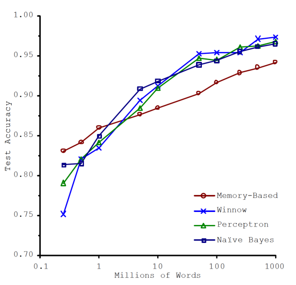
“However, these results suggest that we may want to reconsider the trade-off between spending time and money on algorithm development versus spending it on corpus development algorithms themselves.”

Attribution: Banko and Brill (2001)

Unreasonable Effectiveness of Data

Halevy, Norvig, and Pereira (2009) and Kaplan et al. (2020).

Peter Norvig’s presentation, titled “The Unreasonable Effectiveness of Data,” runs for just over one hour. It is noteworthy that the paper on which the presentation is based was published in 2009, predating the success of AlexNet.

The substantial improvements observed with AlexNet in 2012 highlighted the benefits of training deep neural networks on large image datasets.

Similarly, modern models like GPT, Gemini, Claude, and LLaMA have achieved significant advancements in language capabilities by training on vast amounts of text data, encompassing nearly all written material since the inception of human civilization.

Neural scaling laws describe how the performance of neural networks varies with changes in key factors such as dataset size, number of parameters, and computational cost Kaplan et al. (2020).

Definition

Data augmentation is a technique used to increase the diversity of a dataset by applying various transformations to the existing data.

Purpose: Enhance the robustness and generalization capability of machine learning models.

Data Augmentation (General)

• For Images: Rotations, translations, scaling, flipping, adding noise, etc.
  • How to find ancient geoglyphs using machine learning?, Sakai et al. (2024)
• For Text: Synonym replacement, random insertion, deletion, and swapping of words.

Bioinformatics

These methods modify existing data to create new instances. In bioinformatics, this might involve introducing mutations, shuffling sequences, or applying reverse-complement transformations to augment positive or negative datasets without altering the underlying biological properties.

This challenge occurs not only when data are limited but also when privacy concerns are present.

Synthetic data provides a controlled environment for assessing various effects in computational experiments. For example, researchers can generate datasets with differing levels of noise, such as 1%, 5%, and 10%, and adjust parameters like G+C content to analyze their impacts.

Nevertheless, findings from synthetic data experiments must be validated with real-world datasets to ensure the reliability and applicability of the results.

Statistical Models

• Same composition
  • Shuffle
• Same di-nucleotide frequency
  • “We present results of computer experiments that indicate that several RNAs for which the native state all have lower folding energy than random RNAs of the same length and dinucleotide frequency.” Clote et al. (2005)
• Markov Chains

Data augmentation is inherently specific to the type of data involved. In this context, our focus is on sequence data.

Machine learning models, particularly deep learning architectures, excel at identifying intricate patterns within data. However, as we have seen in the last lecture, their complexity often leads to a propensity for overfitting the training dataset.

This issue is particularly pronounced when employing data augmentation techniques to create negative examples. If not approached with caution, the model may merely learn to differentiate between authentic biological data and artificially generated random data, thereby failing to produce meaningful insights.

Simulation

• Simulation-Based Methods

  • These approaches use mechanistic or rule-based models to emulate underlying biological processes. For example, in silico simulation of sequencing reads, transcription factor binding events, or cellular dynamics can produce realistic synthetic positive examples, while deliberately omitting key features yields negative examples.

  • Trost et al. (2023)

Generative Model-Based Approaches

• Deep learning techniques such as Generative Adversarial Networks (GANs), Variational Autoencoders (VAEs), and autoregressive models learn the statistical distribution of real data to generate new samples.

• Conditional variants allow explicit control over whether the output is a positive or negative example.

• Linder et al. (2020)

Generative Model-Based Approaches

Goyal and Mahmoud (2024)

• “GANs, such as conditional GANs (cGANs) and tabular GANs (TGANs), are particularly susceptible to mode collapse, where the model generates a limited variety of outputs and fails to capture the full diversity of input data.”

• “If the training data are biased, the synthetic data will likely reflect these biases (…)”

See also: Shumailov et al. (2024).

Transfer Learning

• Transfer learning is a machine learning technique that leverages knowledge acquired from one task to enhance performance on a related task.

• This approach minimizes the data and computational resources required for the subsequent task.

Transfer Learning

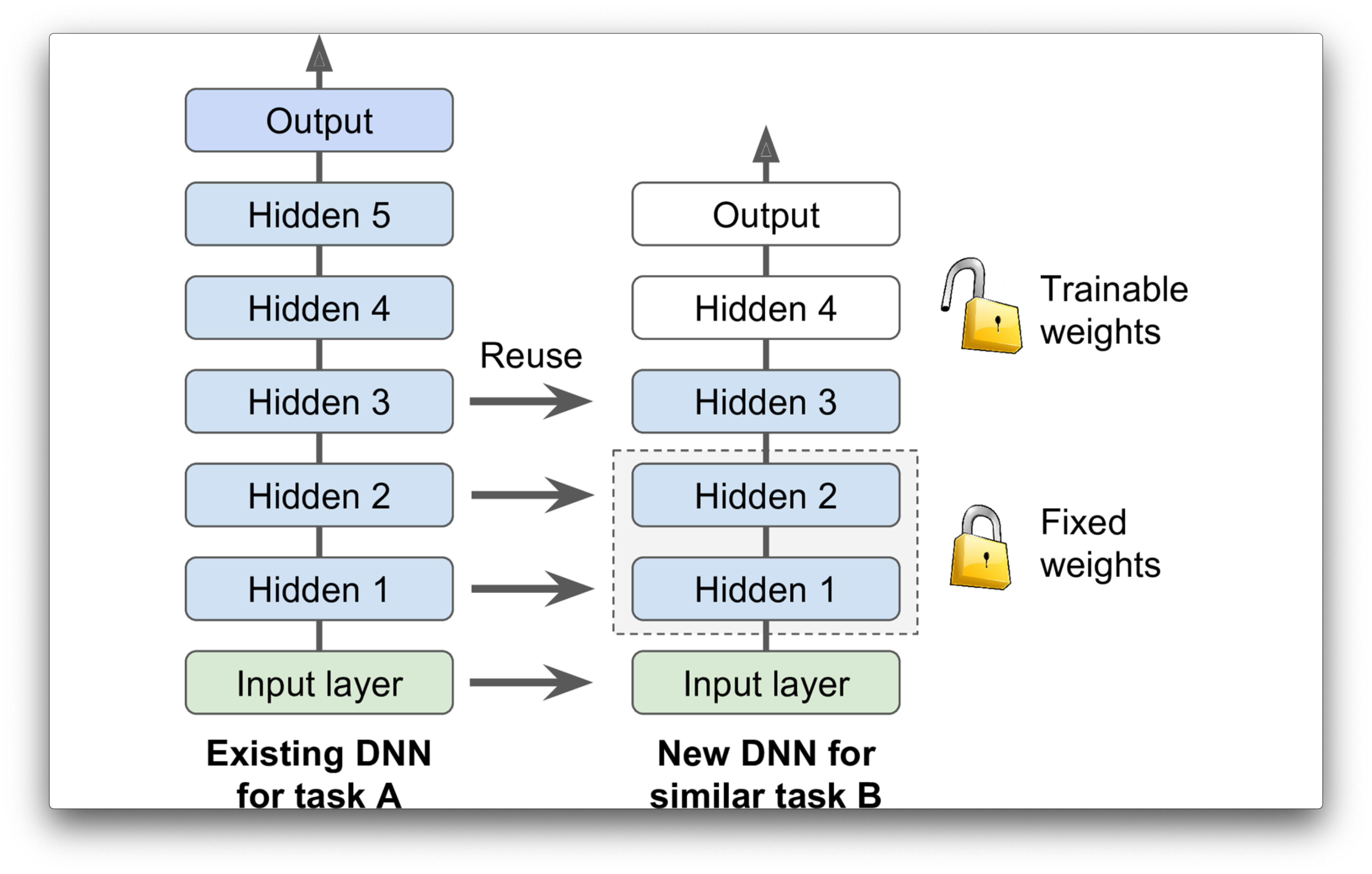
• Transfer learning involves utilizing a substantial segment of a deep neural network, initially trained for a specific task, and making minor adjustments to adapt it for a different task.

  • A primary rationale for transfer learning is to accelerate the training process.

  • A more compelling reason is to enable deep learning applications in domains where the availability of training samples is limited.

Transfer learning

Attribution: Geron (2019) Figure 11.4

Transfer Learning in Bioinformatics

Computational elucidation of membrane protein (MP) structures is challenging partially due to lack of sufficient solved structures for homology modeling. Here, we describe a high-throughput deep transfer learning method that first predicts MP contacts by learning from non-MPs and then predicts 3D structure models using the predicted contacts as distance restraints.

Wang et al. (2017)

Multi-Task Learning

• Multi-task deep learning trains a single model on several related tasks by sharing a common feature extractor with task-specific output layers.

• This shared representation acts as implicit data augmentation and regularization—leveraging additional supervisory signals to boost performance and reduce overfitting, particularly when training data is scarce.

Zhang et al. (2022)

Negative Examples

• Obtaining negative examples is challenging because experiments are generally designed to detect a signal, not confirm its absence.

• Verifying a true negative requires controls that unequivocally rule out an interaction—something that’s inherently difficult to achieve in complex biological systems.

Protein-Protein Interactions

• The protein-protein interaction (PPI) problem focuses on identifying and understanding the physical and functional interactions between proteins within a biological system.

• Yeast-two-hybrid (Y2H) experiments reveal the presence of protein-protein interactions but do not confirm their absence.

• Negative examples typically consist of pairs lacking any evidence of interaction.

Protein-Protein Interactions

• The human genome encodes approximately 20,000 distinct proteins, excluding any potential isoforms.

  • Consequently, the theoretical number of possible protein-protein interactions is approximately 200 million.

  • However, only about 650,000 of these are estimated to be true positives Stumpf et al. (2008), resulting in a significant class imbalance problem with a ratio of approximately 300:1.

“(…) led one study recently published in Bioinformatics to the erroneous conclusion that predictive algorithms based on protein sequence features are hardly better than random in predicting PPIs” Park and Marcotte (2011)

Machine Learning Engineering

Machine Learning Engineering

1. Gather adequate data.
2. Extract features from the raw data:
   • This process is labor-intensive.
   • It necessitates creativity.
   • Domain knowledge is highly beneficial.

Dataset - Adult

import numpy as np
np.random.seed(42)

from sklearn.datasets import fetch_openml

adult = fetch_openml(name='adult', version=2)
print(adult.DESCR)

Author: Ronny Kohavi and Barry Becker
Source: UCI - 1996
Please cite: Ron Kohavi, “Scaling Up the Accuracy of Naive-Bayes Classifiers: a Decision-Tree Hybrid”, Proceedings of the Second International Conference on Knowledge Discovery and Data Mining, 1996

Prediction task is to determine whether a person makes over 50K a year. Extraction was done by Barry Becker from the 1994 Census database. A set of reasonably clean records was extracted using the following conditions: ((AAGE>16) && (AGI>100) && (AFNLWGT>1)&& (HRSWK>0))

This is the original version from the UCI repository, with training and test sets merged.

Variable description

Variables are all self-explanatory except fnlwgt. This is a proxy for the demographic background of the people: “People with similar demographic characteristics should have similar weights”. This similarity-statement is not transferable across the 51 different states.

Description from the donor of the database:

The weights on the CPS files are controlled to independent estimates of the civilian noninstitutional population of the US. These are prepared monthly for us by Population Division here at the Census Bureau. We use 3 sets of controls. These are: 1. A single cell estimate of the population 16+ for each state. 2. Controls for Hispanic Origin by age and sex. 3. Controls by Race, age and sex.

We use all three sets of controls in our weighting program and “rake” through them 6 times so that by the end we come back to all the controls we used. The term estimate refers to population totals derived from CPS by creating “weighted tallies” of any specified socio-economic characteristics of the population. People with similar demographic characteristics should have similar weights. There is one important caveat to remember about this statement. That is that since the CPS sample is actually a collection of 51 state samples, each with its own probability of selection, the statement only applies within state.

Relevant papers

Ronny Kohavi and Barry Becker. Data Mining and Visualization, Silicon Graphics.
e-mail: ronnyk ‘@’ live.com for questions.

Downloaded from openml.org.

Le jeu de données ‘Adult’ contient plusieurs attributs caractérisés par des valeurs catégorielles. Ce jeu de données servira de base pour une brève discussion sur l’encodage de ces valeurs catégorielles.

Adult - Workclass

adult.data['workclass'].unique()

['Private', 'Local-gov', NaN, 'Self-emp-not-inc', 'Federal-gov', 'State-gov', 'Self-emp-inc', 'Without-pay', 'Never-worked']
Categories (8, object): ['Federal-gov', 'Local-gov', 'Never-worked', 'Private', 'Self-emp-inc', 'Self-emp-not-inc', 'State-gov', 'Without-pay']

Adult - Education

adult.data['education'].unique()

['11th', 'HS-grad', 'Assoc-acdm', 'Some-college', '10th', ..., 'Assoc-voc', '9th', '12th', '1st-4th', 'Preschool']
Length: 16
Categories (16, object): ['10th', '11th', '12th', '1st-4th', ..., 'Masters', 'Preschool', 'Prof-school', 'Some-college']

Adult - Marital Status

adult.data['marital-status'].unique()

['Never-married', 'Married-civ-spouse', 'Widowed', 'Divorced', 'Separated', 'Married-spouse-absent', 'Married-AF-spouse']
Categories (7, object): ['Divorced', 'Married-AF-spouse', 'Married-civ-spouse', 'Married-spouse-absent', 'Never-married', 'Separated', 'Widowed']

Categorical Data

Key Points on Data Representation

• Numerical Representation: Some learning algorithms require data to be in numerical form.
• Example Attribute: Consider the workclass attribute, which has 8 distinct values like ‘Federal-gov’, ‘Local-gov’, and so on.

Encoding Methods

Which encoding method is preferable and why?

1. w = 1, 2, 3, 4, 5, 6, 7, or 8
2. w = [0,0,0], [0,0,1], [0,1,0], \(\ldots\), or [1,1,1]
3. w = [1,0,0,0,0,0,0,0], [0,1,0,0,0,0,0,0], \(\ldots\), or [0,0,0,0,0,0,0,1]

Encoding for Categorical Data

One-Hot Encoding: This method should be preferred for categorical data.

• Increases Dimensionality: One-hot encoding increases the dimensionality of feature vectors.
• Avoids Bias: Other encoding methods can introduce biases.
• Example of Bias: Using the first method, w = 1, 2, 3, etc., implies that ‘Federal-gov’ and ‘Local-gov’ are similar, while ‘Federal-gov’ and ‘Without-pay’ are not.
• Misleading Similarity: The second method, w = [0,0,0], [0,0,1], etc., might mislead the algorithm by suggesting similarity based on numeric patterns.

Definition

One-Hot Encoding: A technique that converts categorical variables into a binary vector representation, where each category is represented by a vector with a single ‘1’ and all other elements as ‘0’.

Later, we will consider another encoding called an embedding.

OneHotEncoder

from numpy import array
from sklearn.preprocessing import OneHotEncoder

work = adult.data[['workclass']]

onehot_encoder = OneHotEncoder()

onehot_encoder.fit(work)
values_encoded = onehot_encoder.transform(work)

for i in range(5): print(values_encoded.toarray()[i])

[0. 0. 0. 1. 0. 0. 0. 0. 0.]
[0. 0. 0. 1. 0. 0. 0. 0. 0.]
[0. 1. 0. 0. 0. 0. 0. 0. 0.]
[0. 0. 0. 1. 0. 0. 0. 0. 0.]
[0. 0. 0. 0. 0. 0. 0. 0. 1.]

Consistency is Key: Ensure you use the same encoding on: Validation Set, Test Set, and Production Data.

A student from my research group faced a challenging debugging issue. They mistakenly created a new encoder for the training set using onehot_encoder.fit(X_test['some_attribute']), which produced a vector representation different from the one used during training. Consequently, the results on the training set were poor, while the results on the test set appeared satisfactory.

While Pandas offers a method called get_dummies() for one-hot encoding, it is important to note the following distinctions:

• Category Memory: OneHotEncoder retains the categories it was trained on, whereas get_dummies() does not.
• Consistency in Production: It is crucial to use the same encoding scheme in production as was used during training to ensure accurate results.
• Vector Length Discrepancies: If get_dummies() encounters a different number of categories in new data, it will produce vectors of varying lengths, leading to potential errors.
• Handling Missing Values: When get_dummies() processes missing values, it generates an additional column to accommodate them.

Ensuring consistency in encoding across training, validation, and production datasets is essential to maintain the integrity and accuracy of your machine learning models.

DNA

from numpy import array
import numpy as np

from sklearn.preprocessing import LabelEncoder
from keras.utils import to_categorical

data = ['T','T','C','T','G','G','C','A','C','T','T','G']

values = array(data)

label_encoder = LabelEncoder ()

integer_encoded = label_encoder.fit_transform(values)
data_encoded = to_categorical(integer_encoded)
data_encoded

array([[0., 0., 0., 1.],
       [0., 0., 0., 1.],
       [0., 1., 0., 0.],
       [0., 0., 0., 1.],
       [0., 0., 1., 0.],
       [0., 0., 1., 0.],
       [0., 1., 0., 0.],
       [1., 0., 0., 0.],
       [0., 1., 0., 0.],
       [0., 0., 0., 1.],
       [0., 0., 0., 1.],
       [0., 0., 1., 0.]])

Embeddings

• “An embedding is a trainable dense vector that represents a category.” [Geron2019 § 13]

• With the one hot encoding, we used a sparse encoding with one dimension per category, e.g., A = [1,0,0,0], to avoid creating false associations between categories.

• With embeddings, the philosophy is the other way around, we want categories that are similar to have similar vector representations.

  • The representation is learnt from the data!
  • Initially, each category is assigned a random vector.
  • During learning, gradient descent will make the vector representations of similar categories more similar to one another.

Embeddings

Why?

• A better representation can accelerate learning and make more accurate predictions.
• Embeddings can be reused! [A form of transfer learning]

Word Embeddings

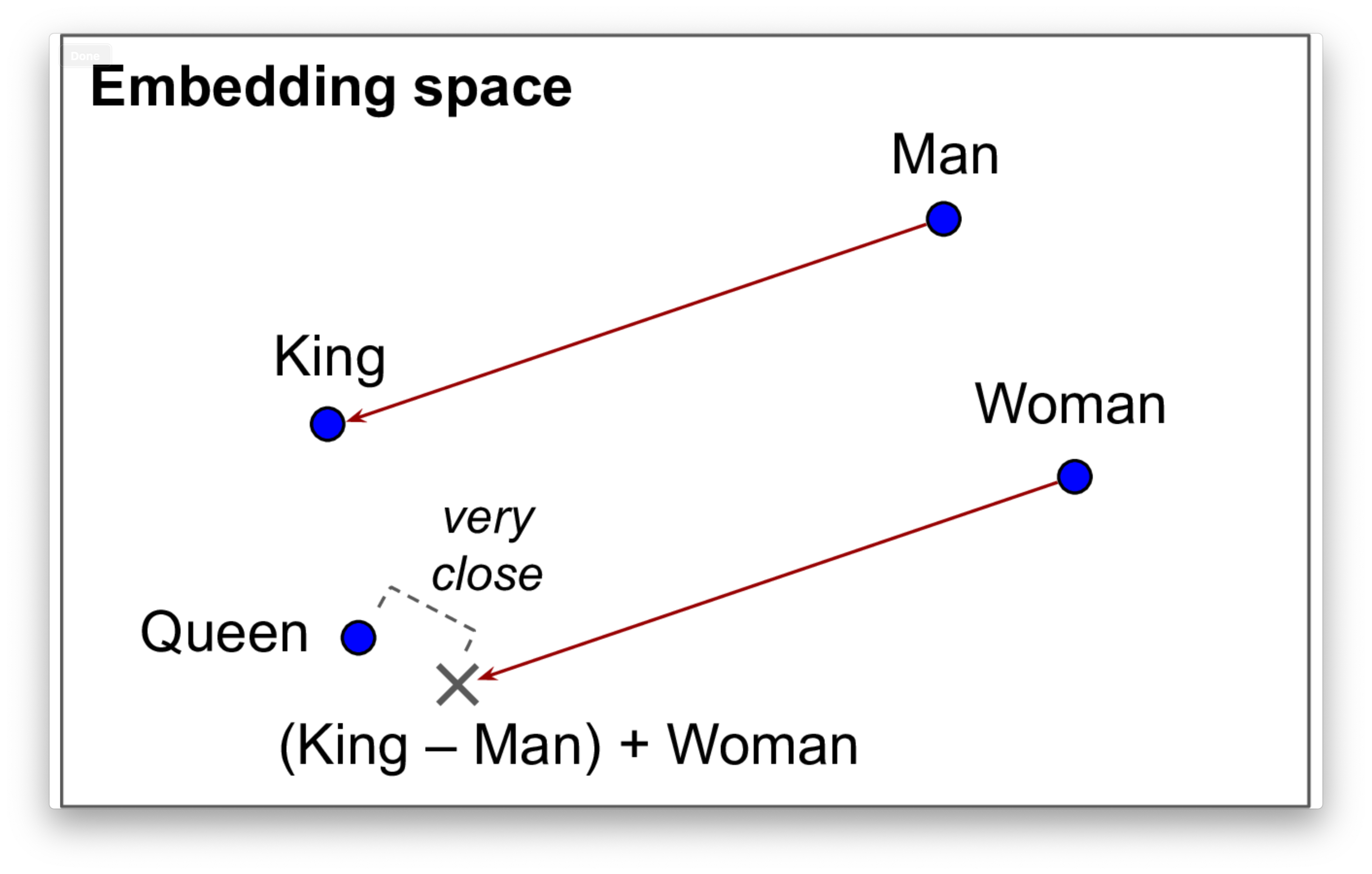
Attribution: [Geron2019] Figure 13.5. “Man is to King as Woman is to Queen”

2013

• Distributed Representations of Words and Phrases and their Compositionality
  • Tomas Mikolov, Ilya Sutskever, Kai Chen, Greg Corrado, Jeffrey Dean
• “Somewhat surprisingly, many of these patterns can be represented as linear translations.”
  • “For example, the result of a vector calculation vec(“Madrid”) - vec(“Spain”) + vec(“France”) is closer to vec(“Paris”) than to any other word vector.”

Embeddings in Bioinformatics

• Bepler, T. & Berger, B. Learning protein sequence embeddings using information from structure. arXiv.org cs.LG, (2019).
• Woloszynek, S., Zhao, Z., Chen, J. & Rosen, G. L. 16S rRNA sequence embeddings: Meaningful numeric feature representations of nucleotide sequences that are convenient for downstream analyses. PLoS Comput Biol 15, (2019).

Embeddings in Bioinformatics

• Asgari, E. & Mofrad, M. R. K. Continuous Distributed Representation of Biological Sequences for Deep Proteomics and Genomics. PLoS ONE 10, (2015).
• Menegaux, R. & Vert, J.-P. Continuous Embeddings of DNA Sequencing Reads and Application to Metagenomics. J Comput Biol 26, cmb.2018.0174–518 (2019).
• Min, X., Zeng, W., Chen, N., Chen, T. & Jiang, R. Chromatin accessibility prediction via convolutional long short-term memory networks with k-mer embedding. Bioinformatics 33, I92–I101 (2017).
• Hamid, M.-N. & Friedberg, I. Identifying Antimicrobial Peptides using Word Embedding with Deep Recurrent Neural Networks. Bioinformatics 25, 3389 (2018).
• Shen, Z., Bao, W. & Huang, D.-S. Recurrent Neural Network for Predicting Transcription Factor Binding Sites. Sci Rep 8, 15270 (2018).

Case Study

Case Study

• Dataset: Heart Disease
  • Examples: 303, features: 13, target: Presence/absence of disease
• Categorical Data:
  • sex: 1 = male, 0 = female
  • cp (chest pain type):
    • 1: Typical angina
    • 2: Atypical angina
    • 3: Non-anginal pain
    • 4: Asymptomatic
  • Other: ‘fbs’, ‘restecg’, ‘exang’, ‘slope’, ‘thal’

To simplify the analysis: Examples with missing values were dropped, no hyperparameter tuning was performed, numerical values were scaled for solver convergence.

Here are some suggestions for further investigation:

• Assess the impact of omitting missing values on the dataset.
• Implement hyperparameter tuning to determine whether \(L_1\) or \(L_2\) regularization enhances model performance.

Case Study

import pandas as pd
import numpy as np
import matplotlib.pyplot as plt
from sklearn.datasets import fetch_openml
from sklearn.preprocessing import OneHotEncoder, StandardScaler
from sklearn.compose import ColumnTransformer
from sklearn.linear_model import LogisticRegression
from sklearn.model_selection import train_test_split
from sklearn.metrics import classification_report

# Load the 'Heart-Disease' dataset from OpenML
data = fetch_openml(name='Heart-Disease', version=1, as_frame=True)
df = data.frame

# Replace '?' with NaN and convert columns to numeric
for col in df.columns:
    df[col] = pd.to_numeric(df[col], errors='coerce')

# Drop rows with missing values
df.dropna(inplace=True)

# Define features and target
X = df.drop(columns=['target'])
y = df['target']

# Columns to encode with OneHotEncoder
columns_to_encode = ['sex', 'cp', 'fbs', 'restecg', 'exang', 'slope', 'thal']

# Identify numerical columns
numerical_columns = X.columns.difference(columns_to_encode)

# Split the dataset into training and testing sets before transformations
X_train, X_test, y_train, y_test = train_test_split(
    X, y, test_size=0.2, random_state=42
)

# Apply OneHotEncoder and StandardScaler using ColumnTransformer
column_transformer = ColumnTransformer(
    transformers=[
        ('onehot', OneHotEncoder(), columns_to_encode),
        ('scaler', StandardScaler(), numerical_columns)
    ]
)

# Fit the transformer on the training data and transform both training and test data
X_train_processed = column_transformer.fit_transform(X_train)
X_test_processed = column_transformer.transform(X_test)

# Initialize and train logistic regression model
model = LogisticRegression(max_iter=1000)
model = model.fit(X_train_processed, y_train)

In the context of using ColumnTransformer, the second element of the triplets, typically an estimator, can also be replaced with the options drop or passthrough. The drop option excludes the specified column from the transformation process, while passthrough retains the column in its original state without any modifications.

Case study - results

# Predict and evaluate the model
y_pred = model.predict(X_test_processed)

print(classification_report(y_test, y_pred))

              precision    recall  f1-score   support

         0.0       0.87      0.93      0.90        29
         1.0       0.93      0.88      0.90        32

    accuracy                           0.90        61
   macro avg       0.90      0.90      0.90        61
weighted avg       0.90      0.90      0.90        61

Case study - chest pain (cp)

# Retrieve feature names after transformation using get_feature_names_out()
feature_names = column_transformer.get_feature_names_out()

# Get coefficients and map them to feature names
coefficients = model.coef_[0]

# Create a DataFrame with feature names and coefficients
coef_df = pd.DataFrame({
    'Feature': feature_names,
    'Coefficient': coefficients
})

# Display coefficients associated with 'cp'
cp_features = coef_df[coef_df['Feature'].str.contains('_cp')]
print("\nCoefficients associated with 'cp':")
print(cp_features)

Coefficients associated with 'cp':
          Feature  Coefficient
2  onehot__cp_0.0    -1.013382
3  onehot__cp_1.0    -0.212284
4  onehot__cp_2.0     0.599934
5  onehot__cp_3.0     0.628824

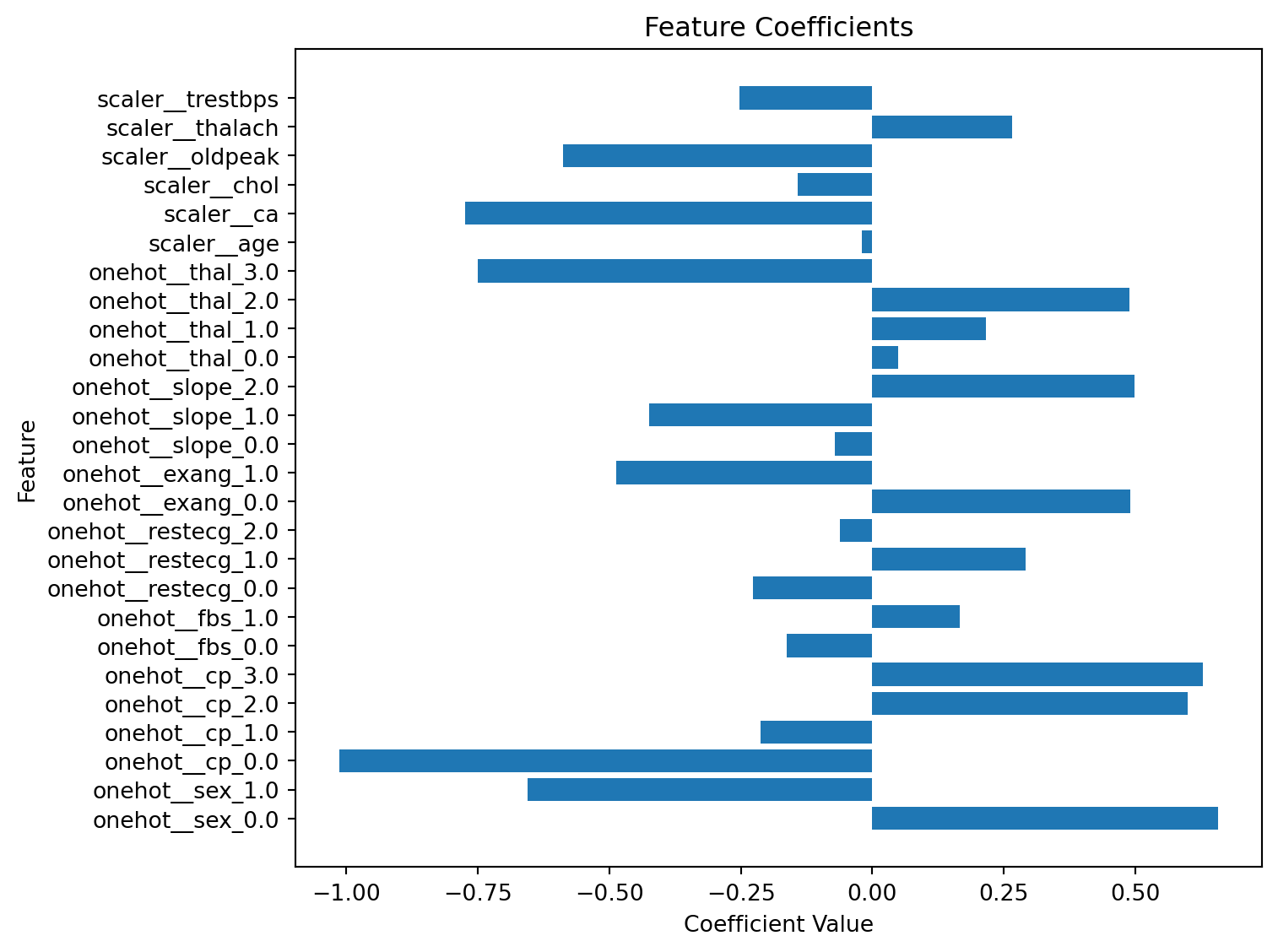
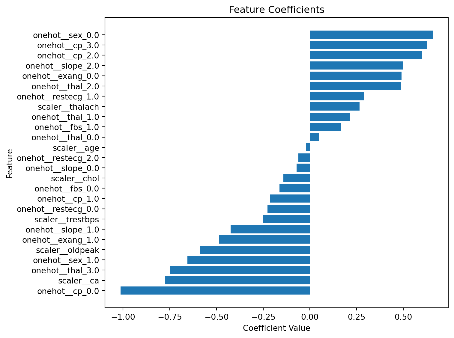
Case study - coefficients

# Visualize the coefficients

plt.figure(figsize=(8, 6))
plt.barh(coef_df['Feature'], coef_df['Coefficient'])
plt.title('Feature Coefficients')
plt.xlabel('Coefficient Value')
plt.ylabel('Feature')
plt.tight_layout()
plt.show()

Positive coefficients in a logistic regression model signify that higher values of the corresponding feature contribute positively to the probability of an example belonging to ‘target = 1.0’. Negative coefficients indicate the opposite effect.

Case study - coefficients (sorted)

# Visualize the coefficients

plt.figure(figsize=(8, 6))
coef_df.sort_values(by='Coefficient', inplace=True)
plt.barh(coef_df['Feature'], coef_df['Coefficient'])
plt.title('Feature Coefficients')
plt.xlabel('Coefficient Value')
plt.ylabel('Feature')
plt.tight_layout()
plt.show()

Definition

Ordinal encoding is a technique that assigns numerical values to categorical attributes based on their inherent order or rank.

Feature Engineering - Ordinal

For attributs with values such as ‘Poor’, ‘Average’, and ‘Good’, an ordinal encoding would make sense.

. . .

However!

from numpy import array
from sklearn.preprocessing import OrdinalEncoder

X =[['Poor'], ['Average'], ['Good'], ['Average'], ['Average']]

encoder = OrdinalEncoder()

encoder.fit(X)
encoder.transform(X)

array([[2.],
       [0.],
       [1.],
       [0.],
       [0.]])

OrdinalEncoder (revised)

from numpy import array
from sklearn.preprocessing import OrdinalEncoder

X =[['Poor'], ['Average'], ['Good'], ['Average'], ['Average']]

encoder = OrdinalEncoder(categories=[['Poor', 'Average', 'Good']])

encoder.fit(X)

X_encoded = encoder.transform(X)

X_encoded

array([[0.],
       [1.],
       [2.],
       [1.],
       [1.]])

The desired order of the categories must be explicitly provided to the encoder; otherwise, it defaults to alphabetical order.

An ordinal encoder is appropriate when categorical attributes have a clear, inherent order or ranking, such as ‘Low’, ‘Medium’, and ‘High’, or ‘Poor’, ‘Average’, and ‘Good’. This encoding method preserves the ordinal relationships among categories.

When data is inherently ordinal, this encoding is more compact and can be advantageous for machine learning models. However, if there is any uncertainty about the ordinal nature of the data, it is safer to use a OneHotEncoder.

Definition

Discretization involves grouping ordinal values into discrete categories.

AKA binning, bucketing, or quantization.

Feature Engineering: Binning

Example: Categorizing ages into bins such as ‘infant’, ‘child’, ‘teen’, ‘adult’, and ‘senior citizen’.

. . .

Advantages:

• Enables the algorithm to learn effectively with fewer training examples.

Disadvantages:

• Requires domain expertise to define meaningful categories.
• May lack generalizability; for example, the starting age for ‘senior citizen’ could be 60, 65, or 70¹.

Providing hints or predefined bins can help a decision tree algorithm generate more compact trees, as it reduces the need for the classifier to independently learn decision boundaries.

However, introducing such a strong bias may hinder the algorithm’s ability to discover meaningful decision boundaries on its own.

Cross-validation is an effective method to determine the best encoding scheme, but it is essential to withhold the test set until the final evaluation phase of the project to prevent data leakage and ensure unbiased assessment.

FunctionTransformer

import pandas as pd
import numpy as np
from sklearn.preprocessing import FunctionTransformer

bins = [0, 1, 13, 20, 60, np.inf]
labels = ['infant', 'kid', 'teen', 'adult', 'senior citizen']

transformer = FunctionTransformer(
    pd.cut, kw_args={'bins': bins, 'labels': labels, 'retbins': False}
)

X = np.array([0.5, 2, 15, 25, 97])
transformer.fit_transform(X)

['infant', 'kid', 'teen', 'adult', 'senior citizen']
Categories (5, object): ['infant' < 'kid' < 'teen' < 'adult' < 'senior citizen']

Se also: KBinsDiscretizer

Scaling

Normalization

Learning algorithms perform optimally when feature values have similar ranges, such as [-1,1] or [0,1].

• This accelerates optimization (e.g., gradient descent).

Normalization: \[ \frac{x_i^{(j)} - \min^{(j)}}{\max^{(j)} - \min^{(j)}} \]

See: sklearn.preprocessing.MinMaxScaler

Standardization

Standardization (AKA z-score normalization) transforms each feature to have a normal distribution with a mean (\(\mu\)) of 0 and a standard deviation (\(\sigma\)) of 1.

\[ \frac{x_i^{(j)} - \mu^{(j)}}{\sigma^{(j)}} \]

Note: The range of values is not bounded!

See: sklearn.preprocessing.StandardScaler

Standardization or Normalization?

• Treat scaling as a hyperparameter and evaluate both normalization and standardization.
• Standardization is generally more robust to outliers than normalization.
• Guidelines from Andriy Burkov (2019), § 5:
  • Use standardization for unsupervised learning tasks.
  • Use standardization if features are approximately normally distributed.
  • Prefer standardization in the presence of outliers.
  • Otherwise, use normalization.

Do you see why standardization is generally more robust to outliers than normalization?

An effective strategy for mitigating the impact of outliers in data is the application of a logarithmic transformation to the values. This technique reduces the skewness of the data, thereby diminishing the disproportionate influence of extreme values.

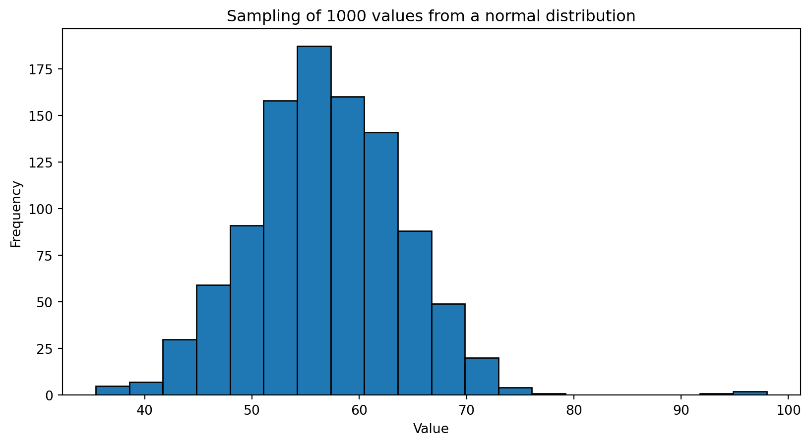
Case Study - Normal Distribution

import numpy as np
np.random.seed(7)

# Sample characteristics
sample_size = 1000
mu = 57
sigma = 7

# Generate values
norm_values = sigma * np.random.randn(sample_size) + mu

# Add three outliers
norm_values = np.append(norm_values, [92, 95, 98])

Case Study - Normal Distribution

Logarithm

Logarithm of values from a normal distribution containing outliers.

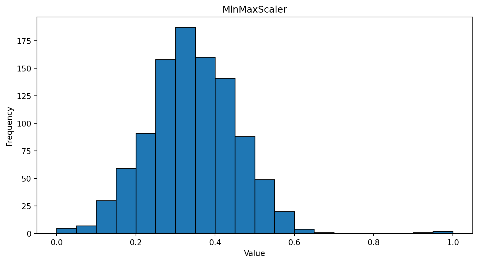
Normalization

Normalization (MinMaxScaler) of values from a normal distribution containing outliers.

Standardization

Standardization (StandardScaler) of values from a normal distribution containing outliers.

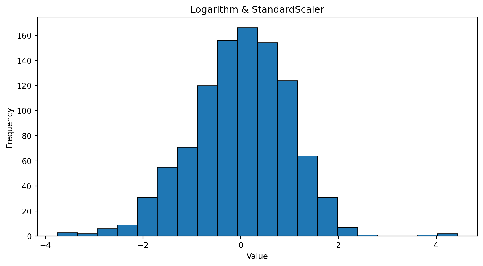
Logarithm & Standardization

Standardization (StandardScaler) of values from a normal distribution containing outliers.

Exponential Distribution

# Sample size
sample_size = 1000

# Generate values
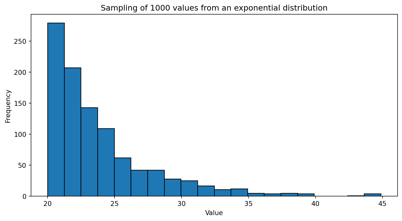
exp_values = np.random.exponential(scale=4, size=sample_size) + 20

In the NumPy expression np.random.exponential(scale=4, size=sample_size) + 20, the parameter scale refers to the inverse rate (or the mean) of the exponential distribution from which the random samples are generated. Specifically, the exponential distribution is defined by its rate parameter, and scale is the reciprocal of this rate, i.e., \(\text{scale} = \frac{1}{\lambda}\).

Thus, scale=4 means that the mean of the exponential distribution is 4. The argument size=sample_size specifies the number of random samples to generate. After generating these samples, 20 is added to each one, thus shifting the entire distribution by 20 units.

Exponential Distribution

Logarithm

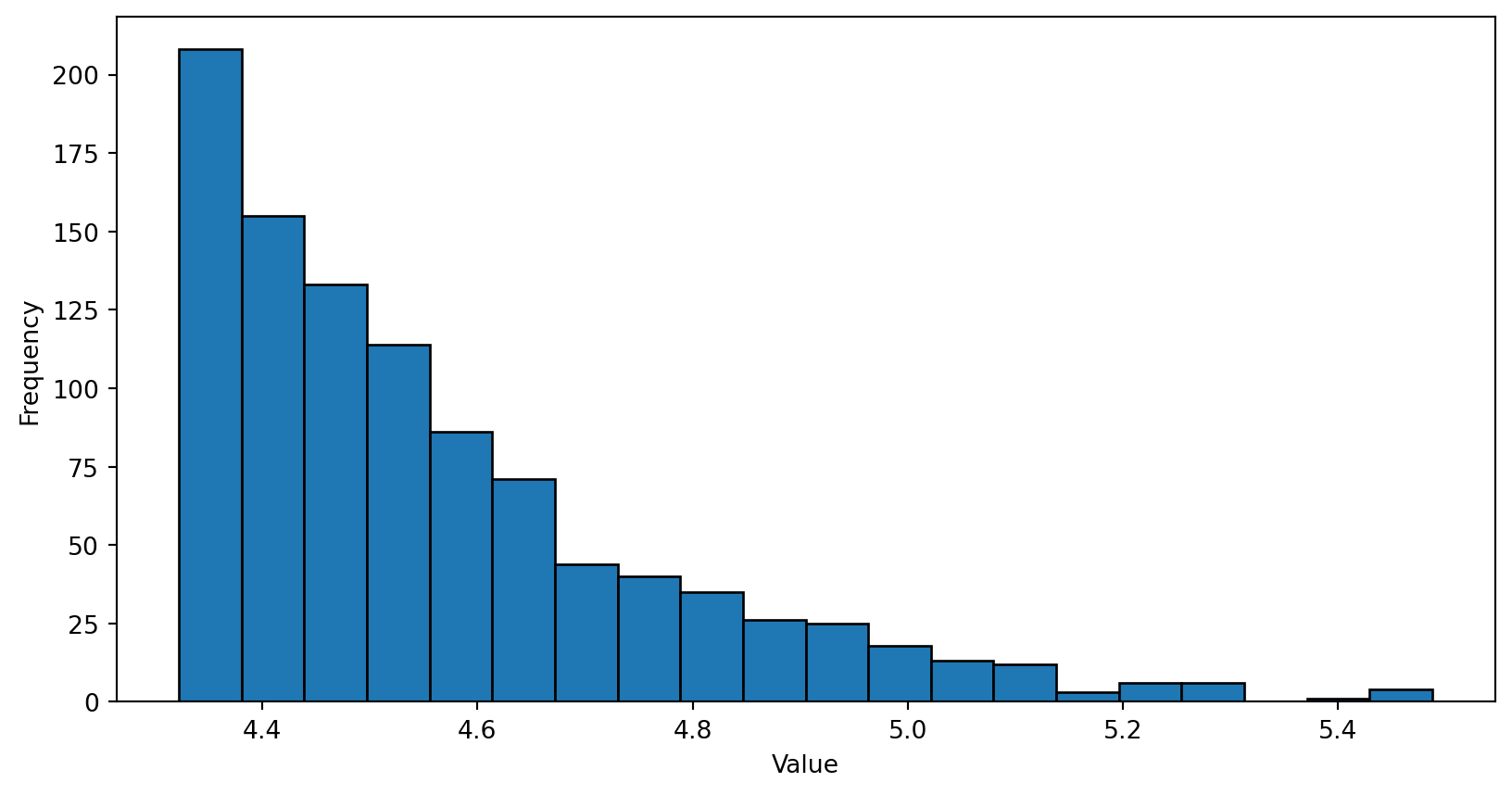
Logarithm of values from an exponential distribution.

Normalization

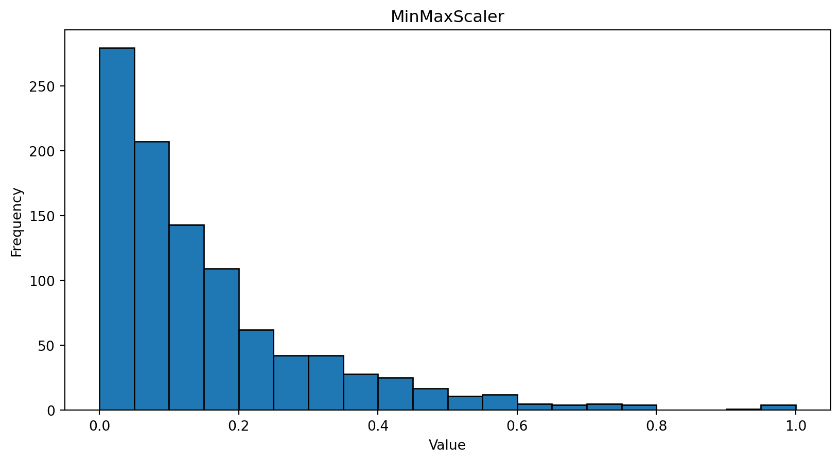
Normalization (MinMaxScaler) of values from an exponential distribution.

Standardization

Standardization (StandardScaler) of values from an exponential distribution.

Logarithm & Standardization

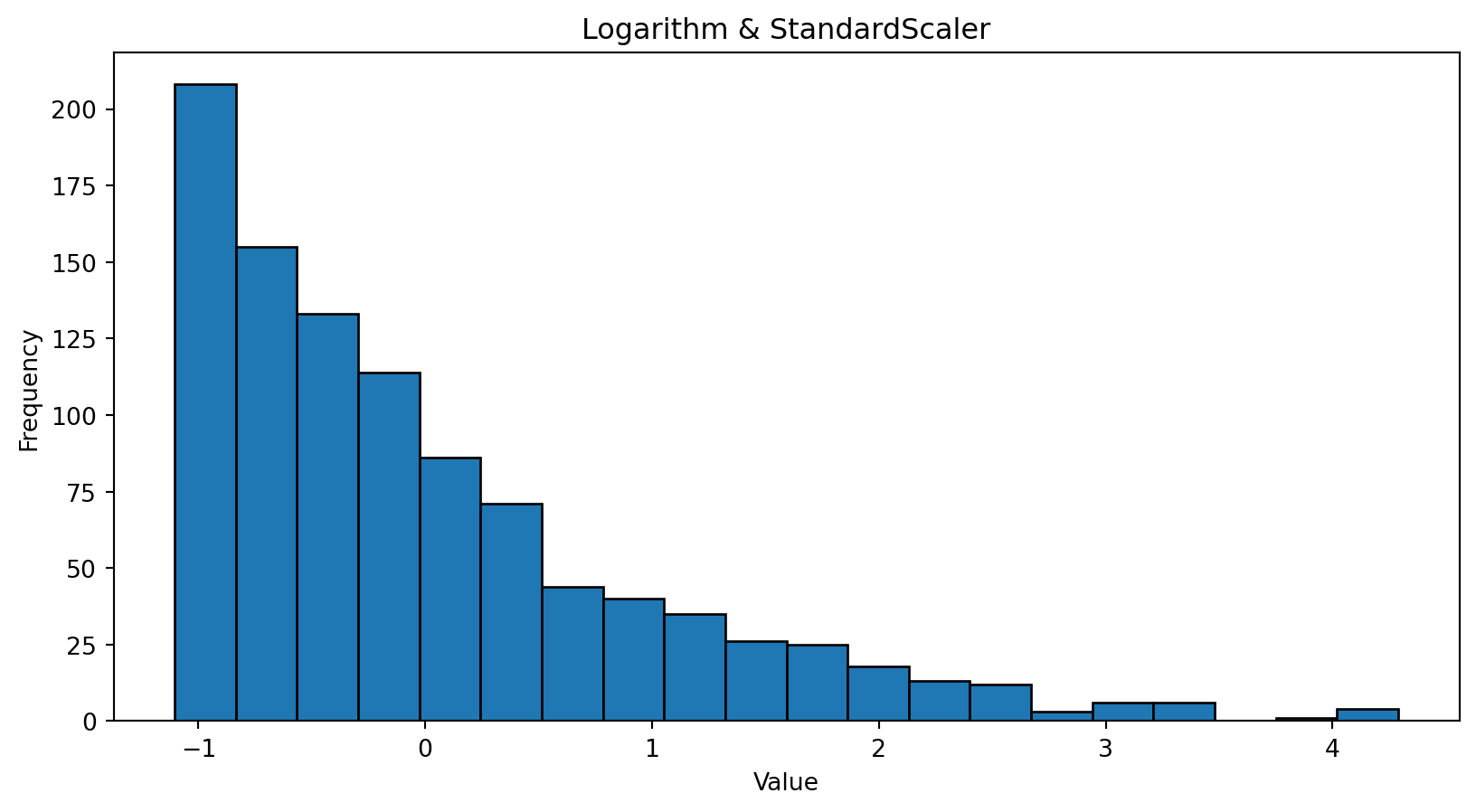
Logarithm and standardization (StandardScaler) of values from an exponential distribution.

Missing Values

Definition

Missing values refer to the absence of data points or entries in a dataset where a value is expected.

Age is a good example, as some patients may withhold their age due to privacy concerns.

Handling Missing Values

• Drop Examples
  • Feasible if the dataset is large and outcome is unaffected.
• Drop Features
  • Suitable if it does not impact the project’s outcome.
• Use Algorithms Handling Missing Data
  • Example: XGBoost
  • Note: Some algorithms like sklearn.linear_model.LinearRegression cannot handle missing values.
• Data Imputation
  • Replace missing values with computed values.

Definition

Data imputation is the process of replacing missing values in a dataset with substituted values, typically using statistical or machine learning methods.

Data Imputation Strategy

Replace missing values with mean or median of the attribute.

from sklearn.impute import SimpleImputer
imputer = SimpleImputer(strategy="median")

X = imputer.fit_transform(X)

. . .

• Cons: Ignores feature correlations and complex relationships.

• Mode Imputation: Replace missing values with the most frequent value; also ignores feature correlations.

Data imputation inherently relies on several assumptions, which may not always hold true.

Randomness Assumption: Many methods (e.g., mean/median imputation) assume that missingness is unrelated to any data.

Model Bias: Incorrect randomness assumptions can lead to biased estimates and flawed conclusions.

Information Loss: Imputation can obscure patterns, leading to loss of valuable information for advanced models.

Proceed with caution!

Data Imputation Strategy

Special Value Method: Replace missing values with a value outside the normal range (e.g., use -1 or 2 for data normalized between [0,1]).

• Objective: Enable the learning algorithm to recognize and appropriately handle missing values.

Data Imputation Strategy

• Middle-Range Imputation: Replace missing values with a value in the middle of the normal range (e.g., use 0 for data distributed in the range [-1,1]).

  • Categorical Data: Use small non-zero numerical values.
    • Example: Use [0.25, 0.25, 0.25, 0.25] instead of [1, 0, 0, 0] for ‘Poor’, [0, 1, 0, 0] for ‘Everage’, [0, 0, 1, 0] for ‘Good’, and [0, 0, 0, 1] for ‘Excellent’.
  • Objective: Minimize the impact of imputed values on the results.

Selection of Method: The effectiveness of imputation methods can vary, and it is essential to compare multiple techniques to determine the best approach for your specific dataset.

Alternative Approach

• Problem Definition: Predict unknown (missing) labels for given examples.
• Have you encountered this kind of problem before?
• Relevance: This can be framed as a supervised learning problem.
  • Let \(\hat{x_i}\) be a new example: \([x_i^{(1)}, x_i^{(2)}, \ldots, x_i^{(j-1)}, x_i^{(j+1)}, \ldots, x_i^{(D)}]\).
  • Let \(\hat{y}_i = x_i^{j}\).
  • Training Set: Use examples where \(x_i^{j}\) is not missing.
  • Method: Train a classifier on this set to predict (impute) the missing values.

Using ML for Imputation

1. Instance-Based Method:

   • Use \(k\) nearest neighbors (k-NN) to find the \(k\) closest examples and impute using the non-missing values from the neighborhood.

2. Model-Based Methods:

   • Employ advanced techniques such as random forests, tensor decomposition, or deep neural networks.

Why Use these Methods?

• Advantages:
  • Effectively handle complex relationships and correlations between features.
• Disadvantages:
  • Cost-intensive in terms of labor, CPU time, and memory resources.

Case Study

• CSI5180: Fundamentals of Machine Learning — Feature Engineering and Data Imputation. Page 34

Class Imbalance

Definition

The class imbablance problem is a scenario where the number of instances in one class significantly outnumbers the instances in other classes.

. . .

Models tend to be biased towards the majority class, leading to poor performance on the minority class.

Standard evaluation metrics like accuracy may be misleading in the presence of class imbalance.

Solutions

• Resampling: Techniques such as oversampling the minority class or undersampling the majority class.

• Algorithmic Adjustments: Using cost-sensitive learning or modifying decision thresholds.

• Synthetic Data: Generating synthetic samples for the minority class using methods like SMOTE (Synthetic Minority Over-sampling Technique).

Apply solutions only to the training set to prevents data leakage.

Chawla et al. (2002) presents the original work, whereas Pradipta et al. (2021) is a recent review.

Oversampling

• Oversampling can lead to overfitting, especially if the synthetic samples are very similar to the existing ones.
• Impact: The model may perform well on training data but generalize poorly to unseen data.

Undersampling

• Loss of Information reduces the number of instances in the majority class.

• Impact: Potentially discards valuable information and can lead to underfitting.

• Reduced Model Performance: Smaller training dataset may not capture the complexity of the problem.

• Impact: Can result in a less accurate and less robust model.

Prologue

Further readings

• Machine Learning Engineering by Andriy Burkov (A. Burkov 2020).
• Covers data collection, storage, preprocessing, feature engineering, model testing and debugging, deployment, retirement, and maintenance.
• From the author of The Hundred-Page Machine Learning Book (Andriy Burkov 2019).
• Available under a “read first, buy later” model.

Summary

• Reviewed data preprocessing techniques: feature engineering, encoding, scaling, and missing value handling.
• Addressed class imbalance and ML pipeline integration.

Next lecture

• Introduction to Deep Learning

References

Banko, Michele, and Eric Brill. 2001. “Scaling to Very Very Large Corpora for Natural Language Disambiguation.” In Proceedings of the 39th Annual Meeting on Association for Computational Linguistics, 26–33. ACL ’01. USA: Association for Computational Linguistics. https://doi.org/10.3115/1073012.1073017.

Burkov, A. 2020. Machine Learning Engineering. True Positive Incorporated. https://books.google.ca/books?id=HeXizQEACAAJ.

Burkov, Andriy. 2019. The Hundred-Page Machine Learning Book. Andriy Burkov.

Chawla, N V, K W Bowyer, L O Hall, and W P Kegelmeyer. 2002. “SMOTE: Synthetic minority over-sampling technique.” Journal of Artificial Intelligence Research 16: 321–57.

Clote, P., F. Ferre, E. Kranakis, and D. Krizanc. 2005. “Structural RNA Has Lower Folding Energy Than Random RNA of the Same Dinucleotide Frequency.” RNA Journal 11 (5): 578–91.

Goyal, Mandeep, and Qusay H. Mahmoud. 2024. “A Systematic Review of Synthetic Data Generation Techniques Using Generative AI.” Electronics 13 (17): 3509. https://doi.org/10.3390/electronics13173509.

Halevy, Alon, Peter Norvig, and Fernando Pereira. 2009. “The Unreasonable Effectiveness of Data.” IEEE Intelligent Systems 24 (2): 8–12.

Kaplan, Jared, Sam McCandlish, Tom Henighan, Tom B. Brown, Benjamin Chess, Rewon Child, Scott Gray, Alec Radford, Jeffrey Wu, and Dario Amodei. 2020. “Scaling Laws for Neural Language Models.” https://arxiv.org/abs/2001.08361.

Linder, Johannes, Nicholas Bogard, Alexander B. Rosenberg, and Georg Seelig. 2020. “A Generative Neural Network for Maximizing Fitness and Diversity of Synthetic DNA and Protein Sequences.” Cell Systems 11 (1): 49–62.e16. https://doi.org/10.1016/j.cels.2020.05.007.

Park, Yungki, and Edward M. Marcotte. 2011. “Revisiting the negative example sampling problem for predicting protein–protein interactions.” Bioinformatics 27 (21): 3024–28. https://doi.org/10.1093/bioinformatics/btr514.

Pradipta, Gede Angga, Retantyo Wardoyo, Aina Musdholifah, I Nyoman Hariyasa Sanjaya, and Muhammad Ismail. 2021. “SMOTE for Handling Imbalanced Data Problem : A Review.” 2021 Sixth International Conference on Informatics and Computing (ICIC) 00: 1–8. https://doi.org/10.1109/icic54025.2021.9632912.

Sakai, Masato, Akihisa Sakurai, Siyuan Lu, Jorge Olano, Conrad M. Albrecht, Hendrik F. Hamann, and Marcus Freitag. 2024. “AI-accelerated Nazca survey nearly doubles the number of known figurative geoglyphs and sheds light on their purpose.” Proceedings of the National Academy of Sciences 121 (40): e2407652121. https://doi.org/10.1073/pnas.2407652121.

Shumailov, Ilia, Zakhar Shumaylov, Yiren Zhao, Nicolas Papernot, Ross Anderson, and Yarin Gal. 2024. “AI models collapse when trained on recursively generated data.” Nature 631 (8022): 755–59. https://doi.org/10.1038/s41586-024-07566-y.

Stumpf, Michael P. H., Thomas Thorne, Eric de Silva, Ronald Stewart, Hyeong Jun An, Michael Lappe, and Carsten Wiuf. 2008. “Estimating the size of the human interactome.” Proceedings of the National Academy of Sciences 105 (19): 6959–64. https://doi.org/10.1073/pnas.0708078105.

Trost, Johanna, Julia Haag, Dimitri Höhler, Laurent Jacob, Alexandros Stamatakis, and Bastien Boussau. 2023. “Simulations of Sequence Evolution: How (Un)realistic They Are and Why.” Molecular Biology and Evolution 41 (1): msad277. https://doi.org/10.1093/molbev/msad277.

Wang, Sheng, Zhen Li, Yizhou Yu, and Jinbo Xu. 2017. “Folding Membrane Proteins by Deep Transfer Learning.” Cell Systems 5 (3): 202–+. https://doi.org/10.1016/j.cels.2017.09.001.

Zaslavsky, Maxim E., Erin Craig, Jackson K. Michuda, Nidhi Sehgal, Nikhil Ram-Mohan, Ji-Yeun Lee, Khoa D. Nguyen, et al. 2025. “Disease diagnostics using machine learning of B cell and T cell receptor sequences.” Science 387 (6736). https://doi.org/10.1126/science.adp2407.

Zhang, Ruiyi, Yunan Luo, Jianzhu Ma, Ming Zhang, and Sheng Wang. 2022. “scPretrain: multi-task self-supervised learning for cell-type classification.” Bioinformatics 38 (6): 1607–14. https://doi.org/10.1093/bioinformatics/btac007.

Appendix: Pipeline

Pipeline

from sklearn.pipeline import Pipeline
from sklearn.preprocessing import StandardScaler

num_pipeline = Pipeline([
        ('imputer', SimpleImputer(strategy="median")),
        ('attribs_adder', CombinedAttributesAdder()),
        ('std_scaler', StandardScaler()),
        ])

training_num_tr = num_pipeline.fit_transform(training_num)

full_pipeline = ColumnTransformer([
        ("num", num_pipeline, num_attribs),
        ("cat", OneHotEncoder(), ["sequence"]),
    ])

training_prepared = full_pipeline.fit_transform(training)

---

Marcel Turcotte

Marcel.Turcotte@uOttawa.ca

School of Electrical Engineering and Computer Science (EECS)

University of Ottawa

Footnotes

1. Your instructor is concerned with your choice of cutoff