Neural networks evolved from simple, biologically inspired perceptrons to deep, multilayer architectures that rely on nonlinear activation functions for learning complex patterns. The universal approximation theorem underpins their ability to approximate any continuous function, and modern frameworks like PyTorch, TensorFlow, and Keras enable practical deep learning applications.
Learning Objectives
Explain basic neural network models (perceptrons and MLPs) and their computational foundations.
Appreciate the limitations of single-layer networks and the necessity for hidden layers.
Describe the role and impact of nonlinear activation functions (sigmoid, tanh, ReLU) in learning.
Articulate the universal approximation theorem and its significance.
Implement and evaluate deep learning models using modern frameworks such as TensorFlow and Keras.
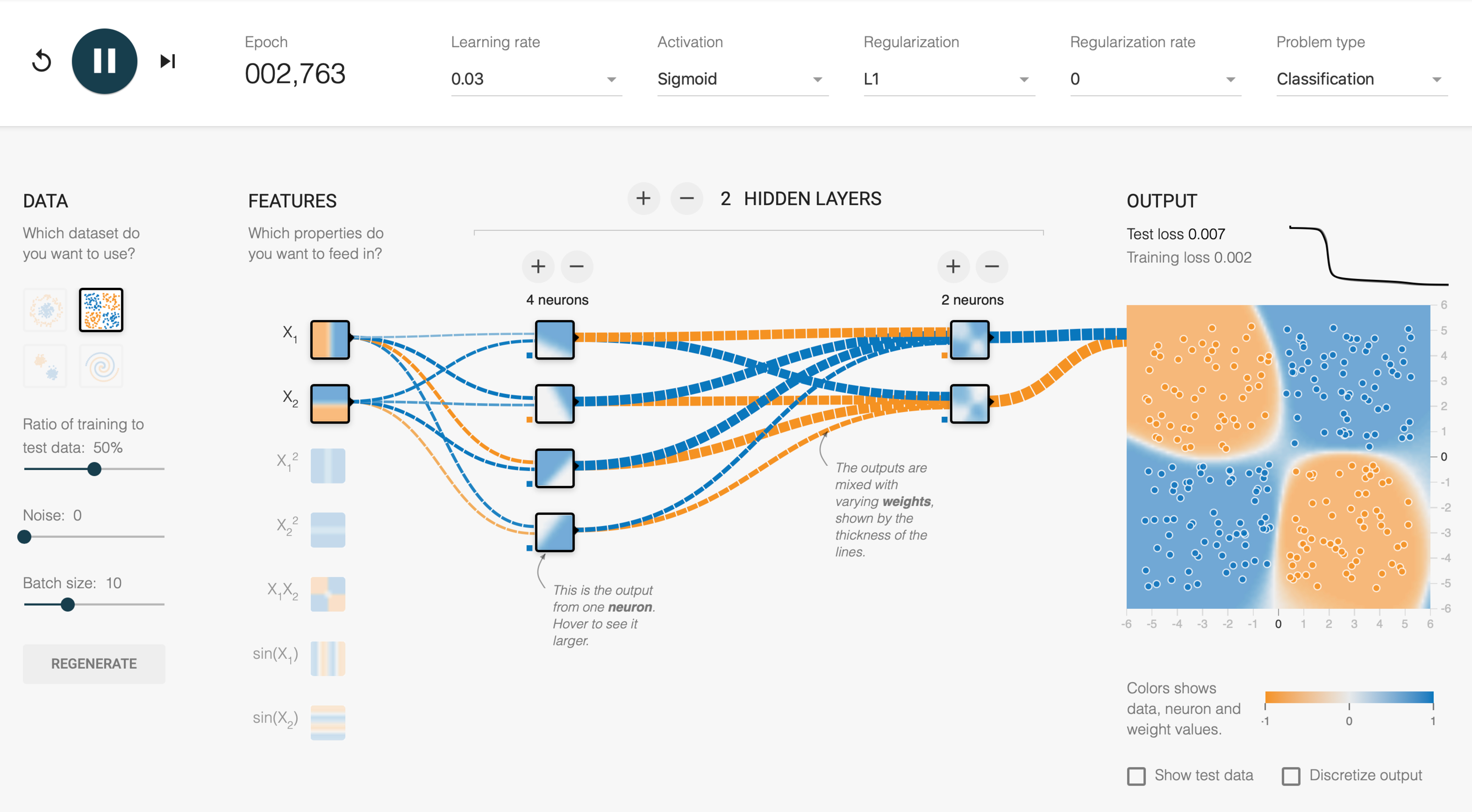
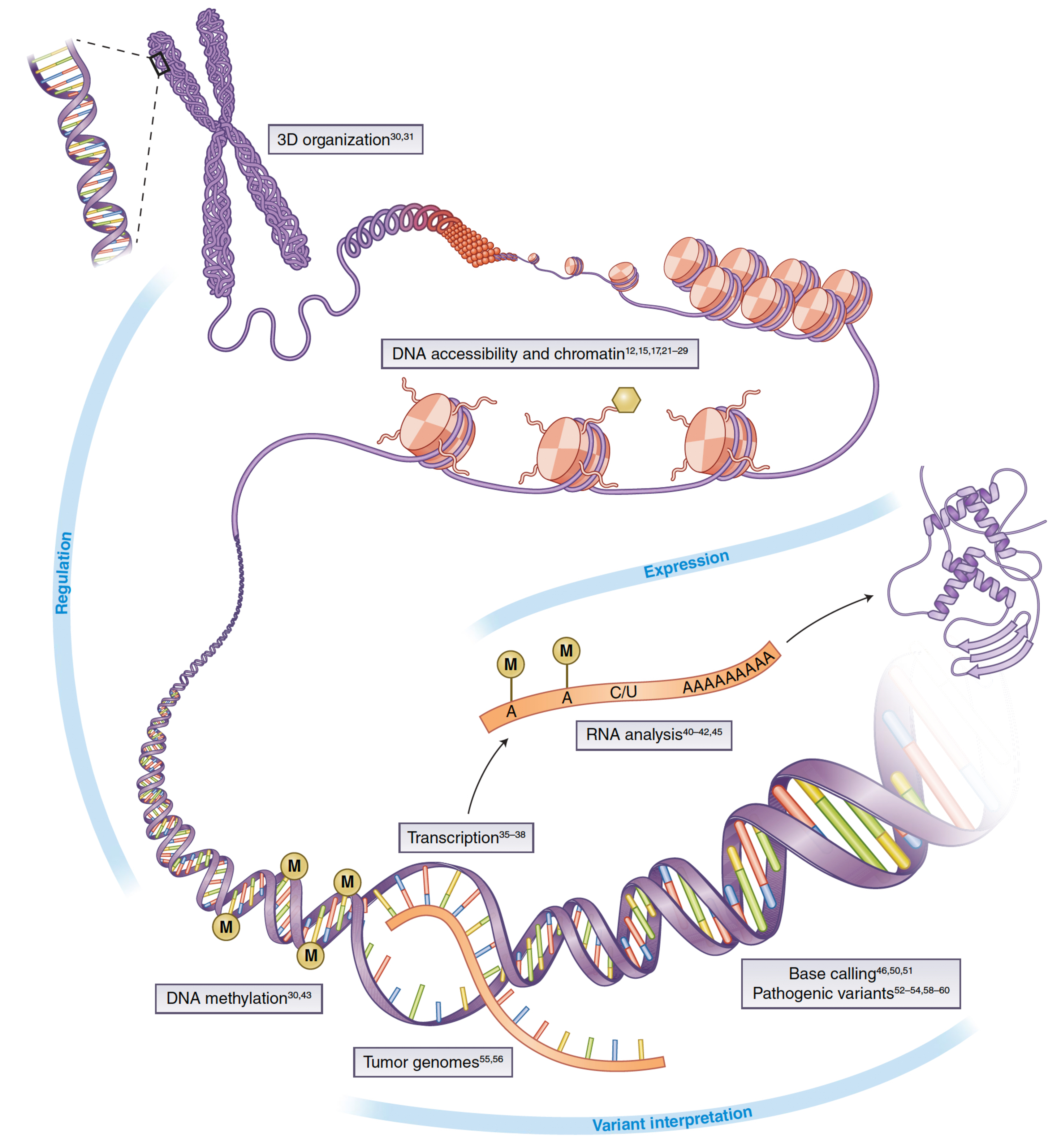
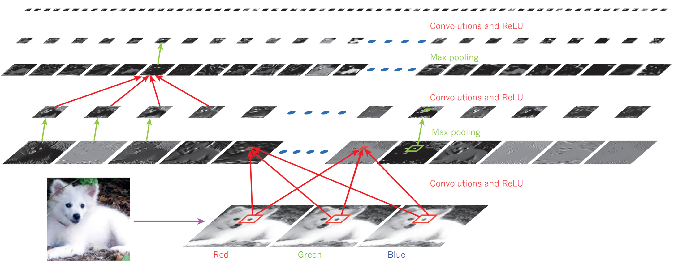
James Zou, Mikael Huss, Abubakar Abid, Pejman Mohammadi, Ali Torkamani, and Amalio Telenti, A primer on deep learning in genomics, Nat Genet51:1, 12–18, 2019.
In the study of artificial intelligence, it is logical to derive inspiration from the most well-understood form of intelligence: the human brain. The brain is composed of a complex network of neurons, which together form biological neural networks. Although each neuron exhibits relatively simple behavior, it is connected to thousands of other neurons, contributing to the intricate functionality of these networks.
A neuron can be conceptualized as a basic computational unit, and the complexity of brain function arises from the interconnectedness of these units.
Yann LeCun and other researchers have frequently noted that artificial neural networks used in machine learning resemble biological neural networks in much the same way that an airplane’s wings resemble those of a bird.
Connectionist
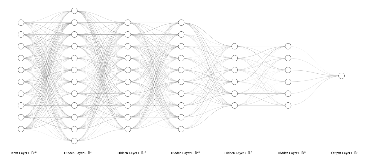
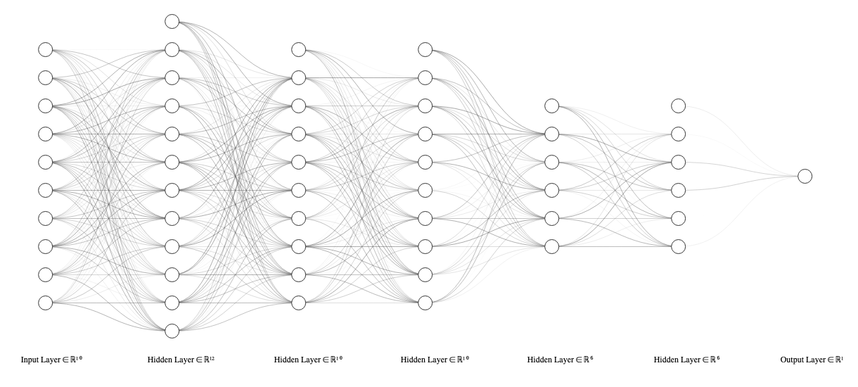
Attribution: LeNail, (2019). NN-SVG: Publication-Ready Neural Network Architecture Schematics. Journal of Open Source Software, 4(33), 747, https://doi.org/10.21105/joss.00747 (GitHub)
A characteristic of biological neural networks that we adopt is the organization of neurons into layers, particularly evident in the cerebral cortex.
Neural networks (NNs) consist of layers of interconnected nodes (neurons), each connection having an associated weight.
Neural networks process input data through these weighted connections, and learning occurs by adjusting the weights based on errors in the training data.
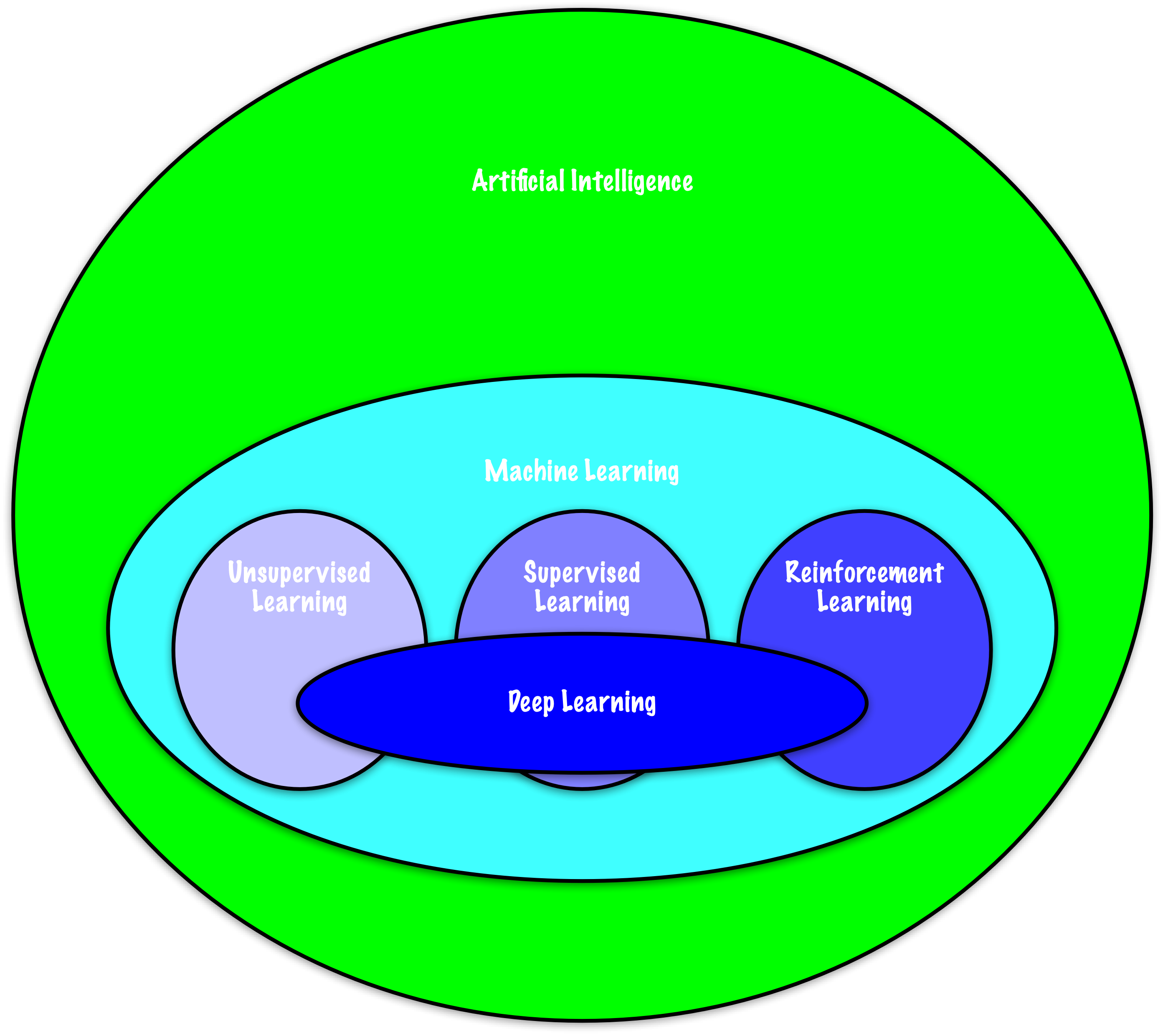
In the book “Deep Learning” (Goodfellow, Bengio, and Courville 2016), authors Goodfellow, Bengio, and Courville define deep learning as a subset of machine learning that enables computers to “understand the world in terms of a hierarchy of concepts.”
This hierarchical approach is one of deep learning’s most significant contributions. It reduces the need for manual feature engineering and redirects the focus toward the engineering of neural network architectures.
Basics
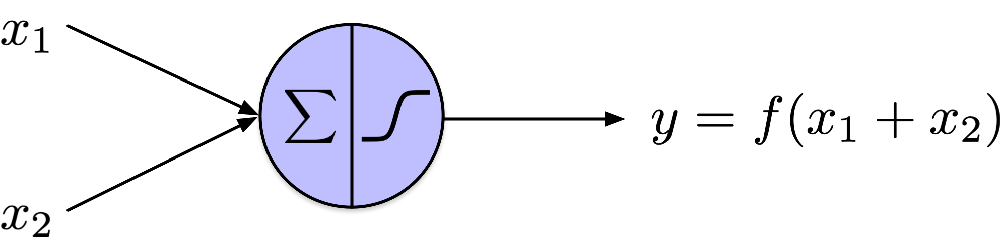
Computations with Neurodes
where \(x_1, x_2 \in \{0,1\}\) and \(f(z)\) is an indicator function:
Neurons can be broadly categorized into two primary types: excitatory and inhibitory.
Computations with Neurodes
Digital computations can be broken down into a sequence of logical operations, enabling neurode networks to execute any computation.
McCulloch and Pitts (1943) did not focus on learning parameter \(\theta\).
They introduced a machine that computes any function but cannot learn.
The period roughly from 1930 to 1950 marked a transformative shift in mathematics toward the formalization of computation. Pioneering work by Gödel, Church, and Turing not only established the theoretical limits and capabilities of computation—with Gödel’s incompleteness theorems, Church’s λ‑calculus and thesis, and Turing’s model of universal machines—but also set the stage for later developments in computer science.
McCulloch and Pitts’ 1943 model of neural networks was inspired by this early mathematical framework linking computation to aspects of intelligence, prefiguring later research in artificial intelligence.
From this work, we take the idea that networks of such units perform computations. Signal propagates from one end of the network to compute a result.
In 1957, Frank Rosenblatt developed a conceptually distinct model of a neuron known as the threshold logic unit, which he published in 1958.
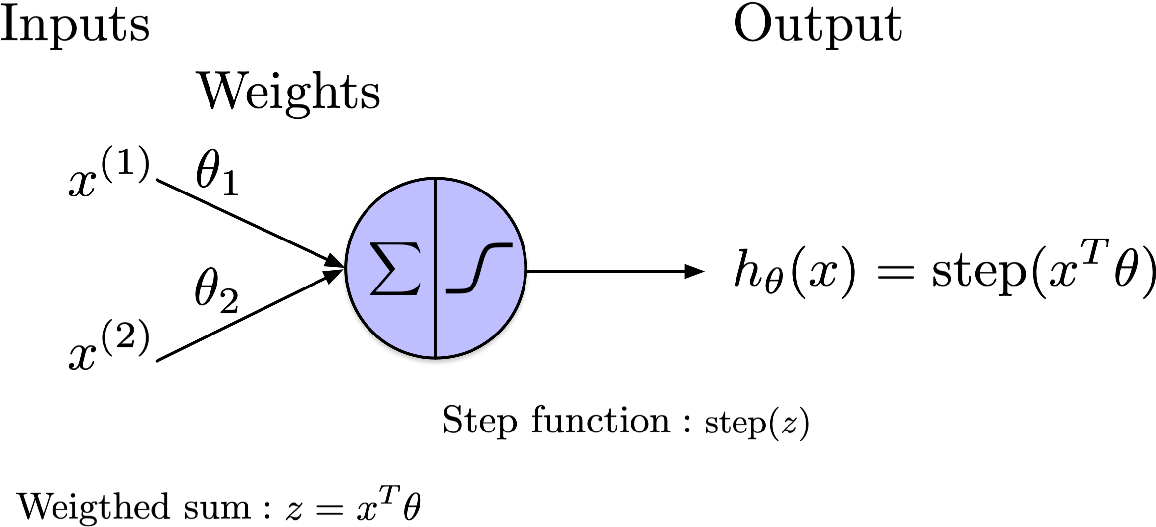
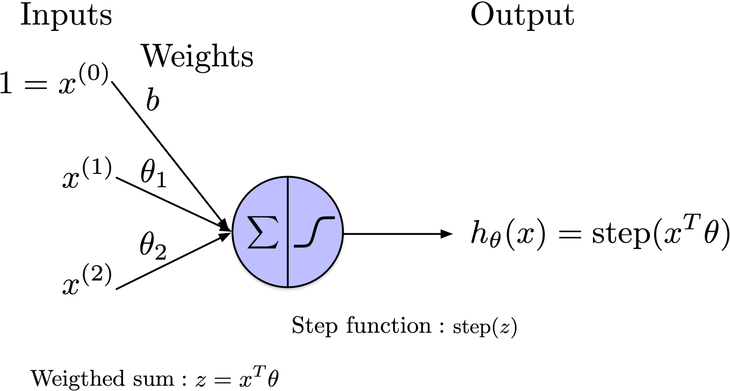
In this model, both the inputs and the output of the neuron are represented as real values. Notably, each input connection has an associated weight.
The left section of the neuron, denoted by the sigma symbol, represents the computation of a weighted sum of its inputs, expressed as \(\theta_1 x_1 + \theta_2 x_2 + \ldots + \theta_D x_D + b\).
This sum is then processed through a step function, right section of the neuron, to generate the output.
Here, \(x^T \theta\) represents the dot product of two vectors: \(x\) and \(\theta\). Here, \(x^T\) denotes the transpose of the vector \(x\), converting it from a row vector to a column vector, allowing the dot product operation to be performed with the vector \(\theta\).
The dot product \(x^T \theta\) is then a scalar given by:
where \(x^{(j)}\) and \(theta_j\) are the components of the vectors \(x\) and \(\theta\), respectively.
Simple Step Functions
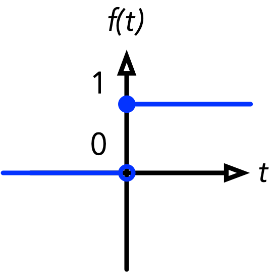
\(\text{heaviside}(t)\) =
1, if \(t \geq 0\)
0, if \(t < 0\)
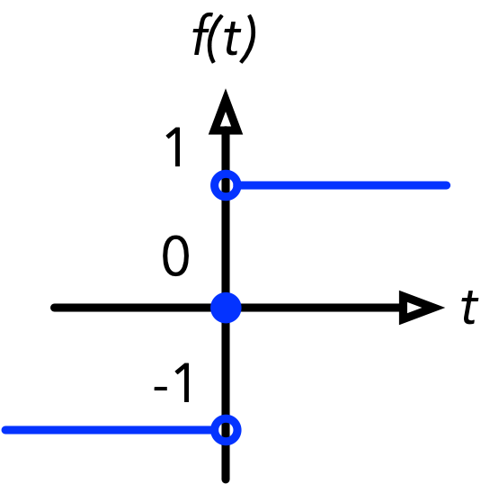
\(\text{sign}(t)\) =
1, if \(t > 0\)
0, if \(t = 0\)
-1, if \(t < 0\)
Common step functions include the heavyside function (0 if the input is negative and 1 otherwise) or the sign function (-1 if the input is negative, 0 if the input is zero, 1 otherwise).
Notation
Add an extra feature with a fixed value of 1 to the input. Associate it with weight \(b = \theta_{0}\), where \(b\) is the bias/intercept term.
Notation
\(\theta_{0} = b\) is the bias/intercept term.
The threshold logic unit is analogous to logistic regression, with the primary distinction being the substitution of the logistic (sigmoid) function with a step function. Similar to logistic regression, the perceptron is employed for classification tasks.
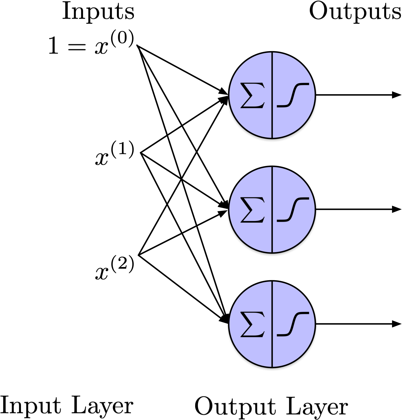
Perceptron
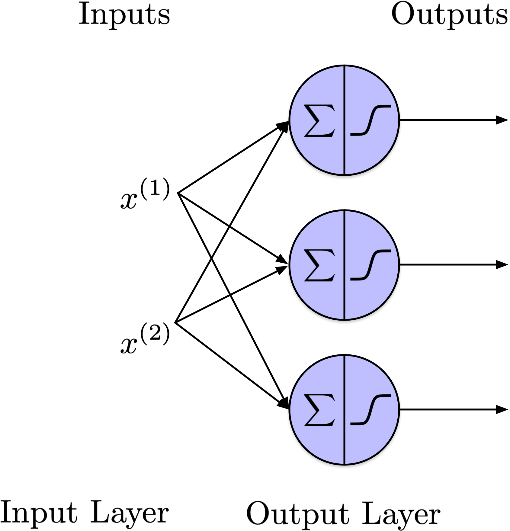
A perceptron consists of one or more threshold logic units arranged in a single layer, with each unit connected to all inputs. This configuration is referred to as fully connected or dense.
Since the threshold logic units in this single layer also generate the output, it is referred to as the output layer.
Perceptron
As this perceptron generates multiple outputs simultaneously, it performs multiple binary predictions, making it as a multilabel classifier (can also be used as multiclass classifier).
Classification tasks, can be further divided into multilabel and multiclass classification.
Multiclass Classification:
In multiclass classification, each instance is assigned to one and only one class out of a set of three or more possible classes. The classes are mutually exclusive, meaning that an instance cannot belong to more than one class at the same time.
Example: Classifying an image as either a cat, dog, or bird. Each image can only belong to one of these categories.
Multilabel Classification:
In multilabel classification, each instance can be associated with multiple classes simultaneously. The classes are not mutually exclusive, allowing for the possibility that an instance can belong to several classes at once.
Example: Tagging an image with multiple attributes such as “outdoor,” “sunset,” and “beach.” The image can simultaneously belong to all these labels.
The key difference lies in the relationship between classes: multiclass classification deals with a single label per instance, while multilabel classification handles multiple labels for each instance.
Notation
As before, introduce an additional feature with a value of 1 to the input. Assign a bias \(b\) to each neuron. Each incoming connection implicitly has an associated weight.
Notation
\(X\) is the input data matrix where each row corresponds to an example and each column represents one of the \(D\) features.
\(W\) is the weight matrix, structured with one row per input (feature) and one column per neuron.
Bias terms can be represented separately; both approaches appear in the literature. Here, \(b\) is a vector with a length equal to the number of neurons.
With neural networks, the parameters of the model are often reffered to as \(w\) (vector) or \(W\) (matrix), rather than \(\theta\).
Discussion
The algorithm to train the perceptron closely resembles stochastic gradient descent.
In the interest of time and to avoid confusion, we will skip this algorithm and focus on multilayer perception (MLP) and its training algorithm, backpropagation.
Historical Note and Justification
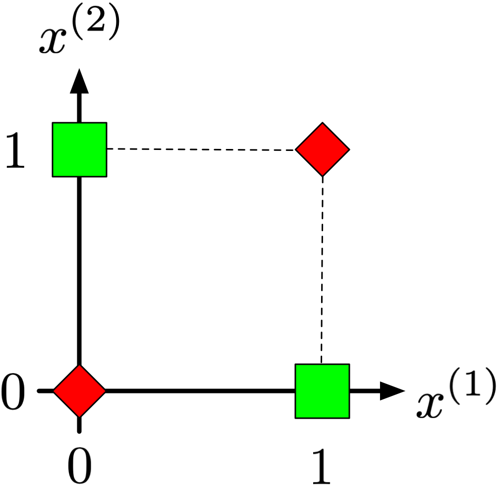
Minsky and Papert (1969) demonstrated the limitations of perceptrons, notably their inability to solve exclusive OR (XOR) classification problems: \({([0,1],\mathrm{true}), ([1,0],\mathrm{true}), ([0,0],\mathrm{false}), ([1,1],\mathrm{false})}\).
This limitation also applies to other linear classifiers, such as logistic regression.
Consequently, due to these limitations and a lack of practical applications, some researchers abandoned the perceptron.
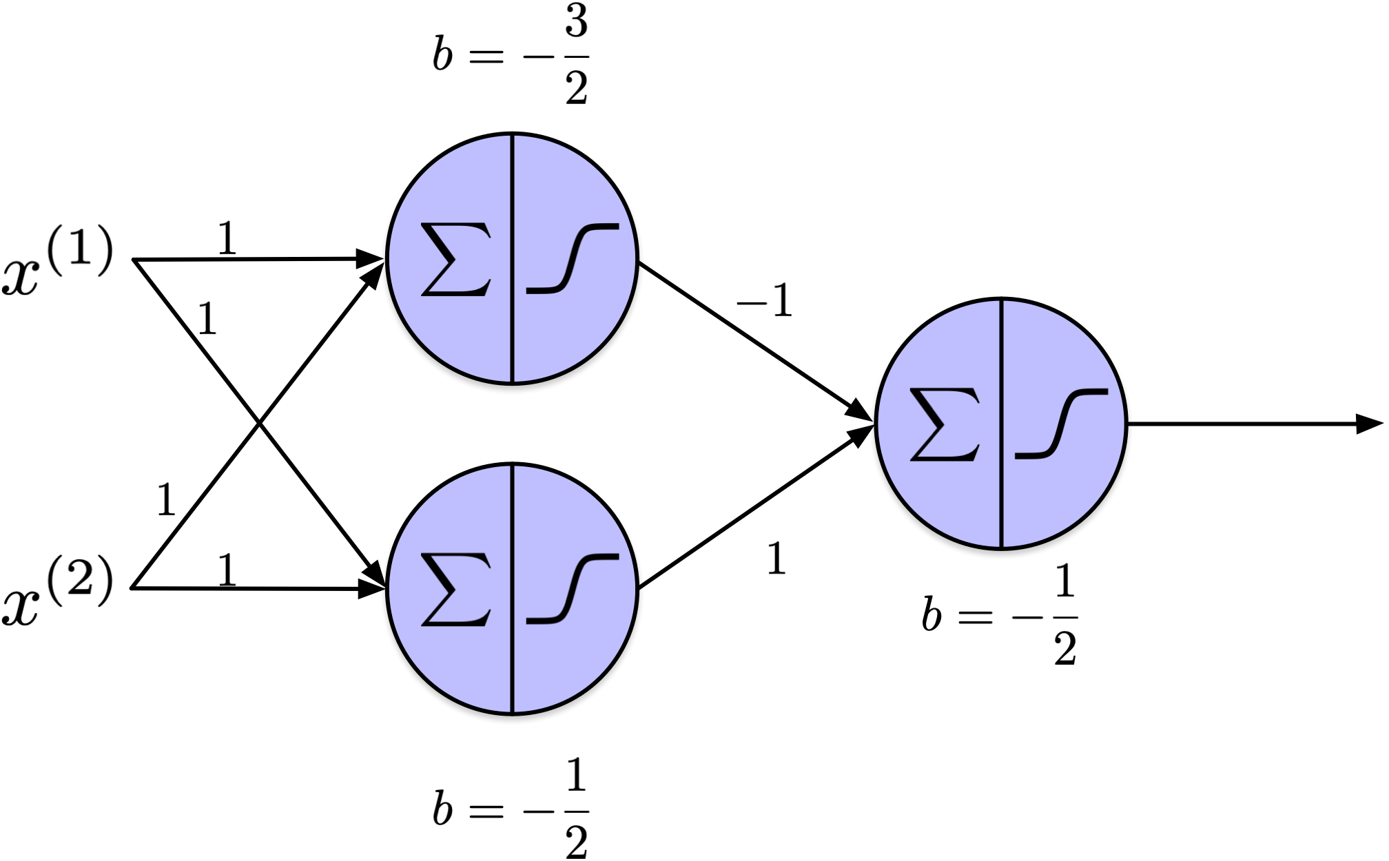
Multilayer Perceptron
A multilayer perceptron (MLP) includes an input layer and one or more layers of threshold logic units. Layers that are neither input nor output are termed hidden layers.
XOR Classification Problem
\(x^{(1)}\)
\(x^{(2)}\)
\(y\)
\(o_1\)
\(o_2\)
\(o_3\)
1
0
1
0
1
1
0
1
1
0
1
1
0
0
0
0
0
0
1
1
0
1
1
0
\(x^{(1)}\) and \(x^{(2)}\) are two attributes, \(y\) is the target, \(o_1\), \(o_2\), and \(o_3 = h_\theta(x)\), are the output of the top left, bottom left, and right threshold units. Clearly \(h_\theta(x) = y, \forall x \in X\). The challenge during Rosenblatt’s time was the lack of algorithms to train multi-layer networks.
I developed an Excel spreadsheet to verify that the proposed multilayer perceptron effectively solves the XOR classification problem.
The step function used in the above model is the heavyside function.
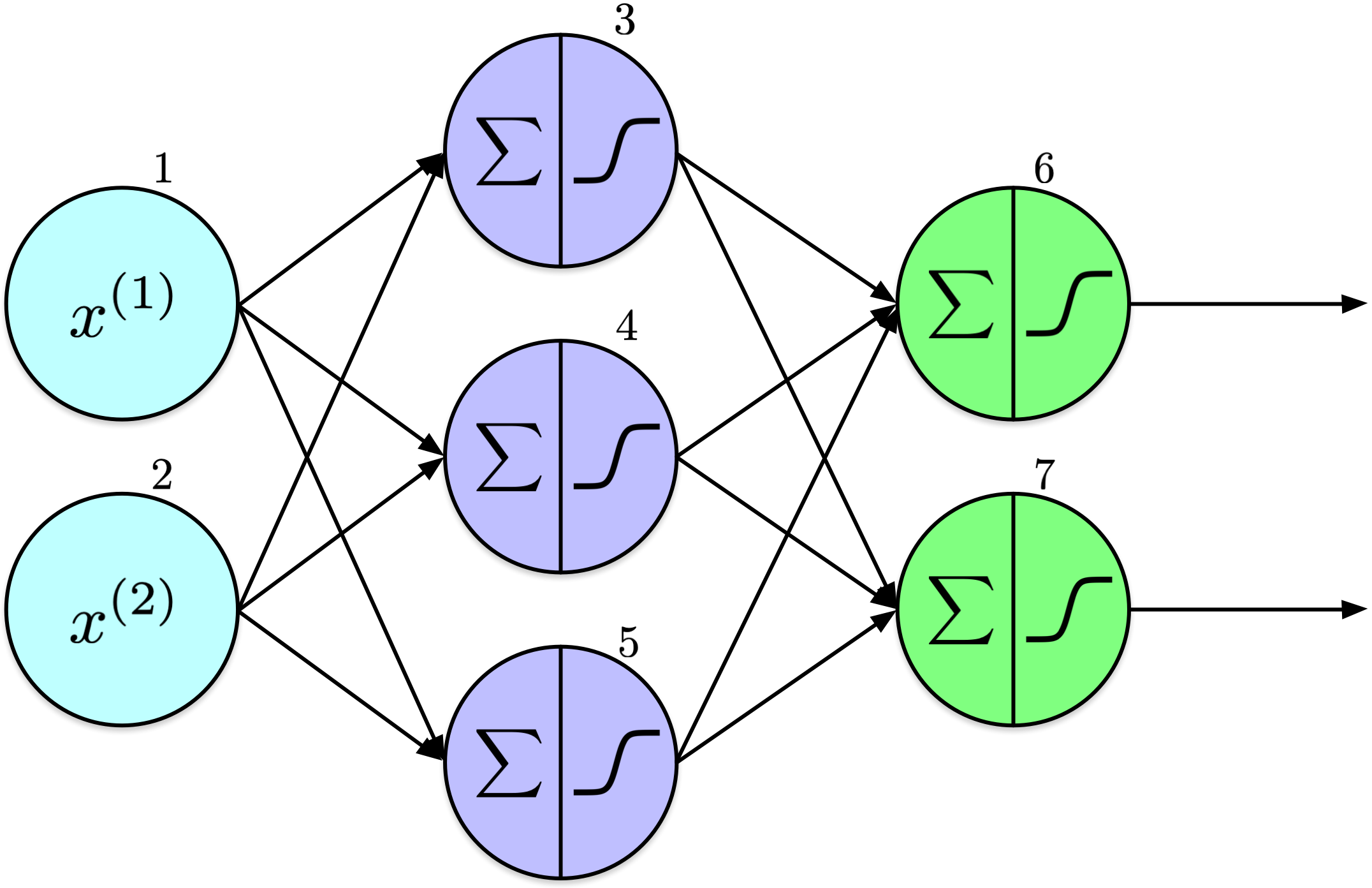
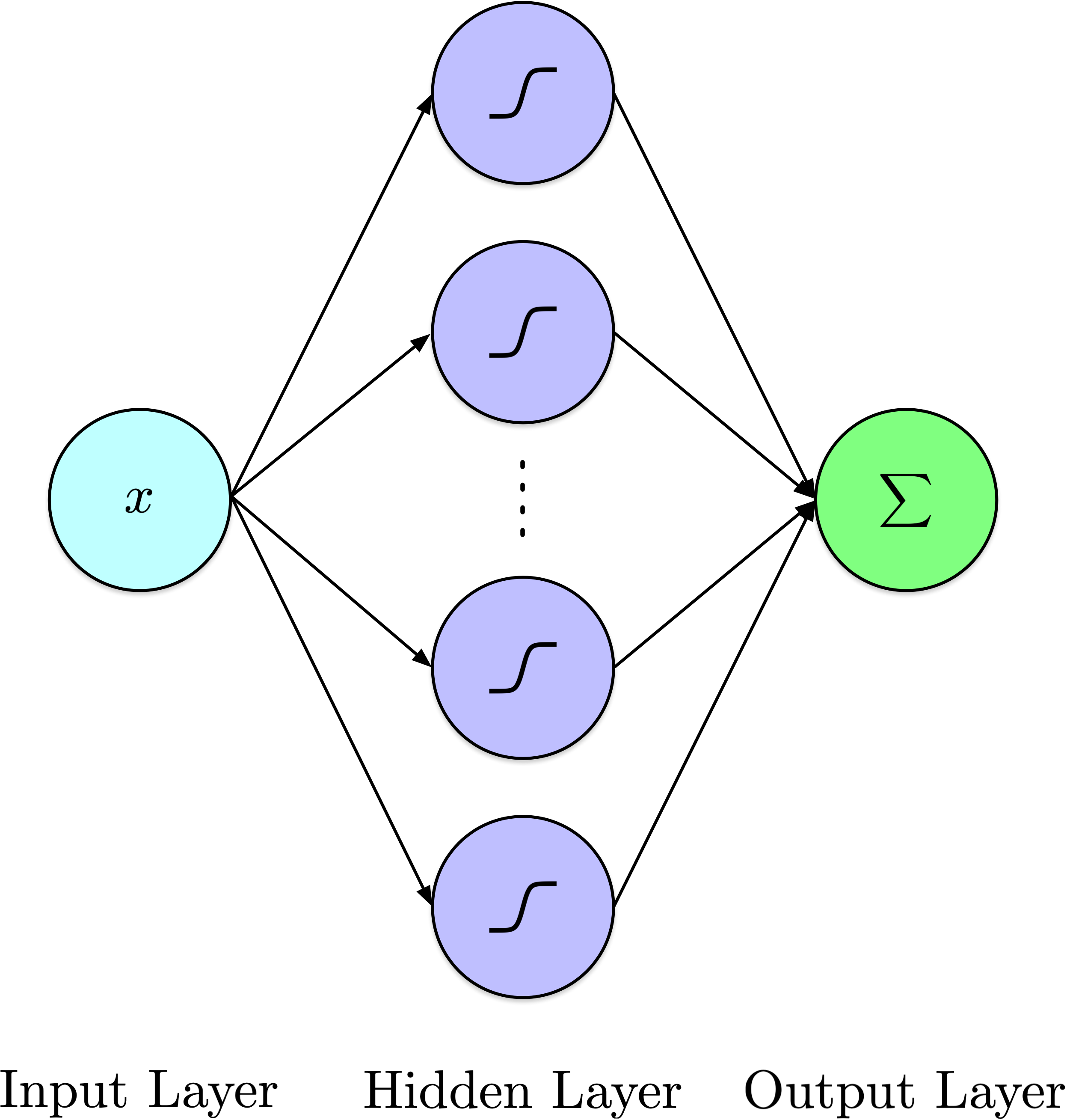
Feedforward Neural Network (FNN)
Information in this architecture flows unidirectionally—from left to right, moving from input to output. Consequently, it is termed a feedforward neural network.
The network consists of three layers: input, hidden, and output. The input layer contains two nodes, the hidden layer comprises three nodes, and the output layer has two nodes. Additional hidden layers and nodes per layer can be added, which will be discussed later.
It is often useful to include explicit input nodes that do not perform calculations, known as input units or input neurons. These nodes act as placeholders to introduce input features into the network, passing data directly to the next layer without transformation. In the network diagram, these are the light blue nodes on the left, labeled 1 and 2. Typically, the number of input units corresponds to the number of features.
For clarity, nodes are labeled to facilitate discussion of the weights between them, such as \(w_{1,5}\) between nodes 1 and 5. Similarly, the output of a node is denoted by \(o_k\), where \(k\) represents the node’s label. For example, for \(k=3\), the output would be \(o_3\).
First, it’s important to understand the information flow: this network computes two outputs from its inputs.
To simplify the figure, I have opted not to display the bias terms, though they remain crucial components. Specifically, \(b_3\) represents the bias term associated with node 3.
If bias terms were not significant, the training process would naturally reduce them to zero. Bias terms are essential as they enable the adjustment of the decision boundary, allowing the model to learn more complex patterns that weights alone cannot capture. By offering additional degrees of freedom, they also contribute to faster convergence during training.
The example above illustrates the computation process with specific values. Before training a neural network, it is standard practice to initialize the weights and biases with random values. Gradient descent is then employed to iteratively adjust these parameters, aiming to minimize the loss function.
Forward Pass (Computatation)
The information flow remains consistent even in more complex networks. Networks with many layers are called deep neural networks (DNN).
As will be discussed later, the training algorithm, known as backpropagation, employs gradient descent, necessitating the calculation of the partial derivatives of the loss function.
The step function in the multilayer perceptron had to be replaced, as it consists only of flat surfaces. Gradient descent cannot progress on flat surfaces due to their zero derivative.
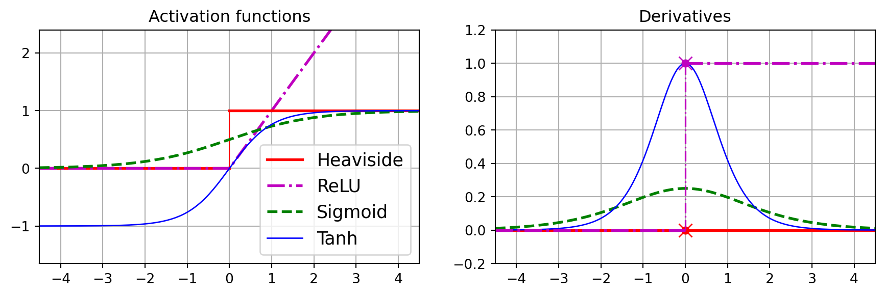
Activation Function
Nonlinear activation functions are paramount because, without them, multiple layers in the network would only compute a linear function of the inputs.
According to the Universal Approximation Theorem, sufficiently large deep networks with nonlinear activation functions can approximate any continuous function. See Universal Approximation Theorem.
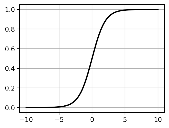
Sigmoid
Code
import numpy as npimport matplotlib.pyplot as plt# Sigmoid functiondef sigmoid(x):return1/ (1+ np.exp(-x))# Generate x valuesx = np.linspace(-10, 10, 400)# Compute y values for the sigmoid functiony = sigmoid(x)plt.figure(figsize=(4,3))plt.plot(x, y, color='black', linewidth=2)plt.grid(True)plt.show()plt.show()
\[
\sigma(t) = \frac{1}{1 + e^{-t}}
\]
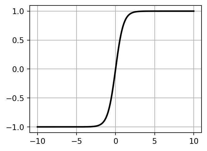
Hyperbolic Tangent Function
Code
# Compute y values for the hyperbolic tangent functiony = np.tanh(x)plt.figure(figsize=(4,3))plt.plot(x, y, color='black', linewidth=2)plt.grid(True)plt.show()
Hyperbolic tangent (\(\tanh(t) = 2 \sigma(2t) - 1\)) is an S-shaped curve, similar to the sigmoid function, producing output values ranging from -1 to 1. According to Géron (2022), this range helps each layer’s output to be approximately centered around 0 at the start of training, thereby accelerating convergence.
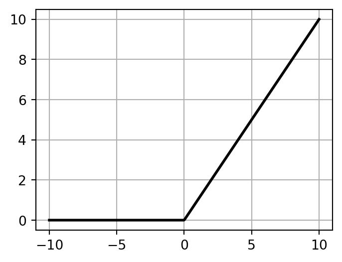
Rectified linear unit function (ReLU)
Code
# Compute y values for the rectified linear unit function (ReLU) functiony = np.maximum(0, x)plt.figure(figsize=(4,3))plt.plot(x, y, color='black', linewidth=2)plt.grid(True)plt.show()
Although the ReLU function (\(\mathrm{ReLU}(t) = \max(0, t)\)) is not differentiable at \(t=0\) and has a derivative of 0 for \(t<0\), it performs quite well in practice and is computationally efficient. Consequently, it has become the default activation function.
The Universal Approximation Theorem (UAT) states that a feedforward neural network with a single hidden layer containing a finite number of neurons can approximate any continuous function on a compact subset of \(\mathbb{R}^n\), given appropriate weights and activation functions.
Cybenko (1989); Hornik, Stinchcombe, and White (1989)
In mathematical terms, a subset of \(\mathbb{R}^n\) is considered compact if it is both closed and bounded.
Closed: A set is closed if it contains all its boundary points. In other words, it includes its limit points or accumulation points.
Bounded: A set is bounded if there exists a real number (M) such that the distance between any two points in the set is less than \(M\).
In the context of the universal approximation theorem, compactness ensures that the function being approximated is defined on a finite and well-behaved region, which is crucial for the theoretical guarantees provided by the theorem.
Single Hidden Layer
\[
y = \sum_{i=1}^N \alpha_i \sigma(w_{1,i} x + b_i)
\]
Notation adapted to follow that of Cybenko (1989).
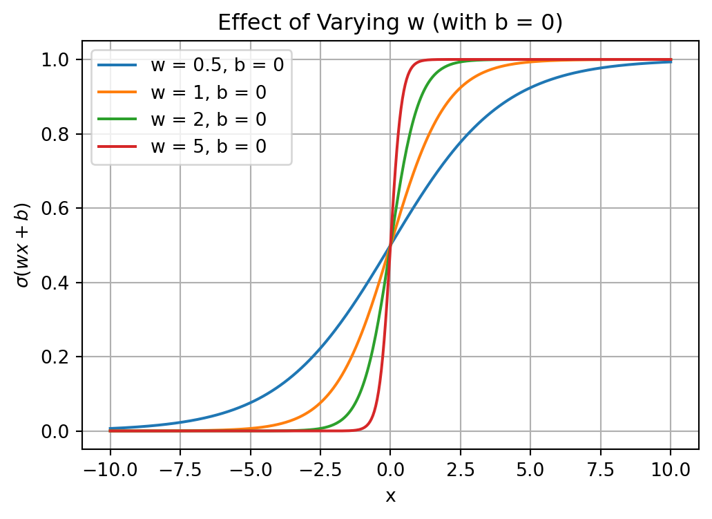
Effect of Varying w
Code
def logistic(x, w, b):"""Compute the logistic function with parameters w and b."""return1/ (1+ np.exp(-(w * x + b)))# Define a range for x values.x = np.linspace(-10, 10, 400)# Plot 1: Varying w (steepness) with b fixed at 0.plt.figure(figsize=(6,4))w_values = [0.5, 1, 2, 5] # different steepness valuesb =0# fixed biasfor w in w_values: plt.plot(x, logistic(x, w, b), label=f'w = {w}, b = {b}')plt.title('Effect of Varying w (with b = 0)')plt.xlabel('x')plt.ylabel(r'$\sigma(wx+b)$')plt.legend()plt.grid(True)plt.show()
Sigmoid activation function: \(\sigma(wx+b)\).
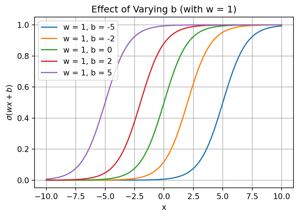
Effect of Varying b
Code
# Plot 2: Varying b (horizontal shift) with w fixed at 1.plt.figure(figsize=(6,4))w =1# fixed steepnessb_values = [-5, -2, 0, 2, 5] # different bias valuesfor b in b_values: plt.plot(x, logistic(x, w, b), label=f'w = {w}, b = {b}')plt.title('Effect of Varying b (with w = 1)')plt.xlabel('x')plt.ylabel(r'$\sigma(wx+b)$')plt.legend()plt.grid(True)plt.show()
Sigmoid activation function: \(\sigma(wx+b)\).
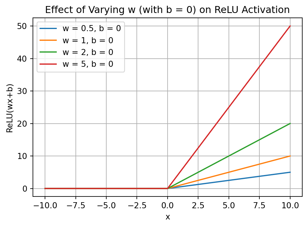
Effect of Varying w
Code
def relu(x, w, b):"""Compute the ReLU activation with parameters w and b."""return np.maximum(0, w * x + b)# Define a range for x values.x = np.linspace(-10, 10, 400)# Plot 1: Varying w (scaling) with b fixed at 0.plt.figure(figsize=(6,4))w_values = [0.5, 1, 2, 5] # different scaling valuesb =0# fixed biasfor w in w_values: plt.plot(x, relu(x, w, b), label=f'w = {w}, b = {b}')plt.title('Effect of Varying w (with b = 0) on ReLU Activation')plt.xlabel('x')plt.ylabel('ReLU(wx+b)')plt.legend()plt.grid(True)plt.show()
ReLU activation function: np.maximum(0, w * x + b).
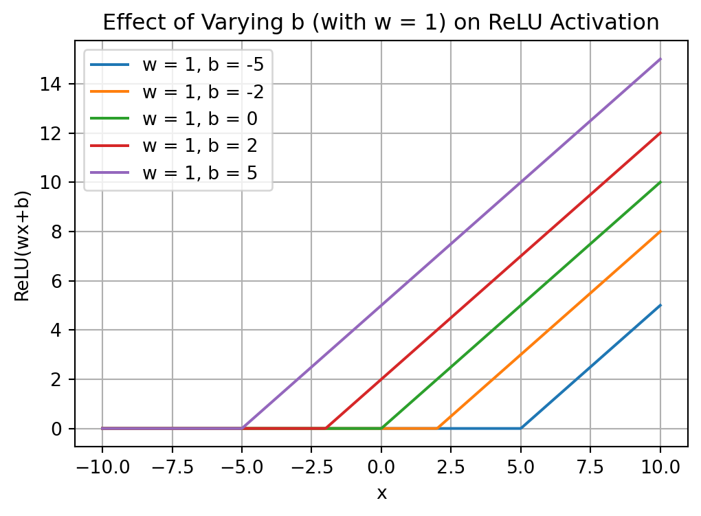
Effect of Varying b
Code
# Plot 2: Varying b (horizontal shift) with w fixed at 1.plt.figure(figsize=(6,4))w =1# fixed scalingb_values = [-5, -2, 0, 2, 5] # different bias valuesfor b in b_values: plt.plot(x, relu(x, w, b), label=f'w = {w}, b = {b}')plt.title('Effect of Varying b (with w = 1) on ReLU Activation')plt.xlabel('x')plt.ylabel('ReLU(wx+b)')plt.legend()plt.grid(True)plt.show()
ReLU activation function: np.maximum(0, w * x + b).
Single Hidden Layer
\[
y = \sum_{i=1}^N \alpha_i \sigma(w_{1,i} x + b_i)
\]
# Defining the function to be approximateddef f(x):return2* x**3+4* x**2-5* x +1# Generating a dataset, x in [-4,2), f(x) as aboveX =6* np.random.rand(1000, 1) -4y = f(X).flatten()
Increasing the Number of Neurons
from sklearn.neural_network import MLPRegressorfrom sklearn.model_selection import train_test_splitX_train, X_valid, y_train, y_valid = train_test_split(X, y, test_size=0.1, random_state=42)models = []sizes = [1, 2, 5, 10, 100]for i, n inenumerate(sizes): models.append(MLPRegressor(hidden_layer_sizes=[n], max_iter=5000, random_state=42)) models[i].fit(X_train, y_train)
MLPRegressor is a multi-layer perceptron regressor from sklearn. Its default activation function is relu.
Increasing the Number of Neurons
Code
# Create a colormapcolors = plt.colormaps['cool'].resampled(len(sizes))X_valid = np.sort(X_valid,axis=0)for i, n inenumerate(sizes): y_pred = models[i].predict(X_valid) plt.plot(X_valid, y_pred, "-", color=colors(i), label="Number of neurons = {}".format(n))y_true = f(X_valid)plt.plot(X_valid, y_true, "r.", label='Actual')plt.legend()plt.show()
In the example above, I retained only 10% of the data as the test set because the function being approximated is straightforward and noise-free. This decision was made to ensure that the true curve does not overshadow the other results.
Increasing the Number of Neurons
Code
for i, n inenumerate(sizes): plt.plot(models[i].loss_curve_, "-", color=colors(i), label="Number of neurons = {}".format(n))plt.title('MLPRegressor Loss Curves')plt.xlabel('Iterations')plt.ylabel('Loss')plt.legend()plt.show()
As expected, increasing neuron count reduces loss.
Universal Approximation
This video effectively conveys the underlying intuition of the universal approximation theorem. (18m 53s)
The video effectively elucidates key concepts (terminology) in neural networks, including nodes, layers, weights, and activation functions. It demonstrates the process of summing activation outputs from a preceding layer, akin to the aggregation of curves. Additionally, the video illustrates how scaling an output by a weight not only alters the amplitude of a curve but also inverts its orientation when the weight is negative. Moreover, it clearly depicts the function of bias terms in vertically shifting the curve, contingent on the sign of the bias.
PyTorch has gained considerable traction in the research community. Initially developed by Meta AI, it is now part of the Linux Foundation.
TensorFlow, created by Google, is widely adopted in industry for deploying models in production environments.
Keras
Keras is a high-level API designed to build, train, evaluate, and execute models across various backends, including PyTorch, TensorFlow, and JAX, Google’s high-performance platform.
As highlighted in previous Quotes of the Day, François Chollet, a Google engineer, is the originator and one of the primary developers of the Keras project.
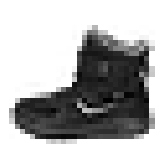
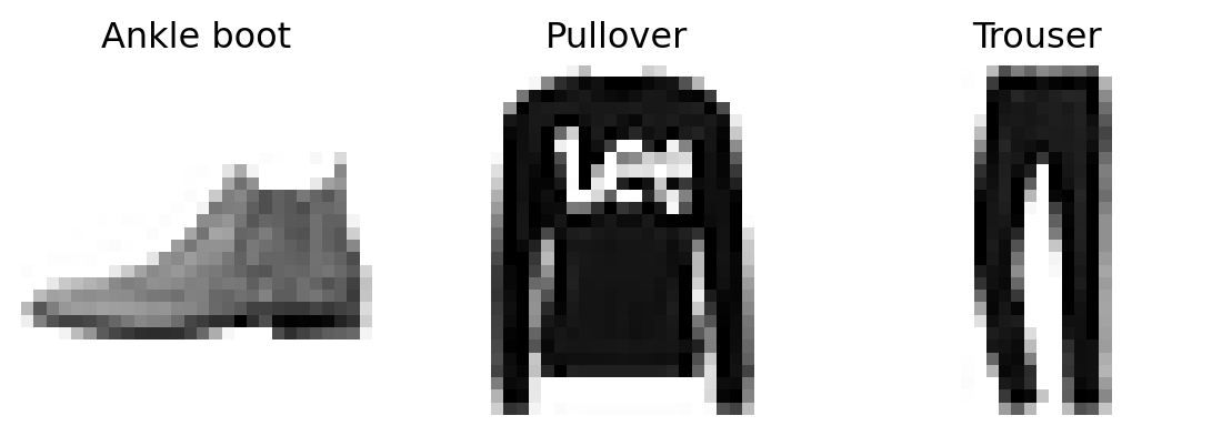
Fashion-MNIST dataset
“Fashion-MNIST is a dataset of Zalando’s article images—consisting of a training set of 60,000 examples and a test set of 10,000 examples. Each example is a 28x28 grayscale image, associated with a label from 10 classes.”
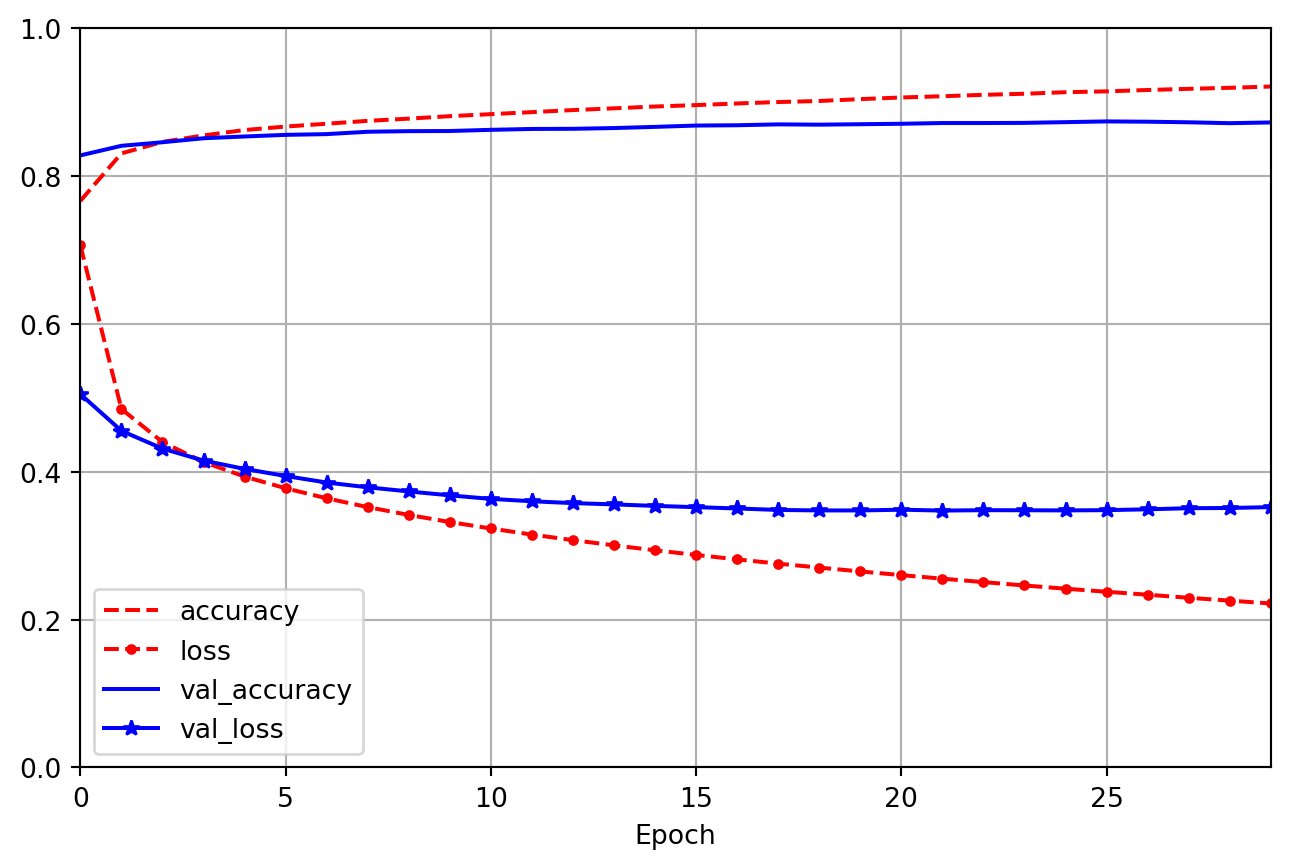
The model is provided with both a taining set and a validation set. At each step, the model will report its performance on both sets. This will also allow to visualize the accuracy and loss curves on both sets (more later).
When calling the fit method in Keras (or similar frameworks), each step corresponds to the evaluation of a mini-batch. A mini-batch is a subset of the training data, and during each step, the model updates its weights based on the error calculated from this mini-batch.
An epoch is defined as one complete pass through the entire training dataset. During an epoch, the model processes multiple mini-batches until it has seen all the training data once. This process is repeated for a specified number of epochs to optimize the model’s performance.
Neural Networks Foundations:
We introduced bio-inspired computation with neurodes and threshold logic units, outlining the perceptron model and its limitations (e.g., the XOR problem).
From Perceptrons to Deep Networks:
We explained the evolution to multilayer perceptrons (MLPs) and feedforward architectures, emphasizing the critical role of nonlinear activation functions (sigmoid, tanh, ReLU) in enabling gradient-based learning and complex function approximation.
Universal Approximation:
We discussed how even single hidden layer networks can approximate any continuous function on a compact set, highlighting the theoretical underpinning of deep learning.
Practical Frameworks and Applications:
Finally, we reviews leading deep learning frameworks (PyTorch, TensorFlow, Keras) and demonstrates practical model-building using the Fashion-MNIST dataset, covering model training, evaluation, and prediction.
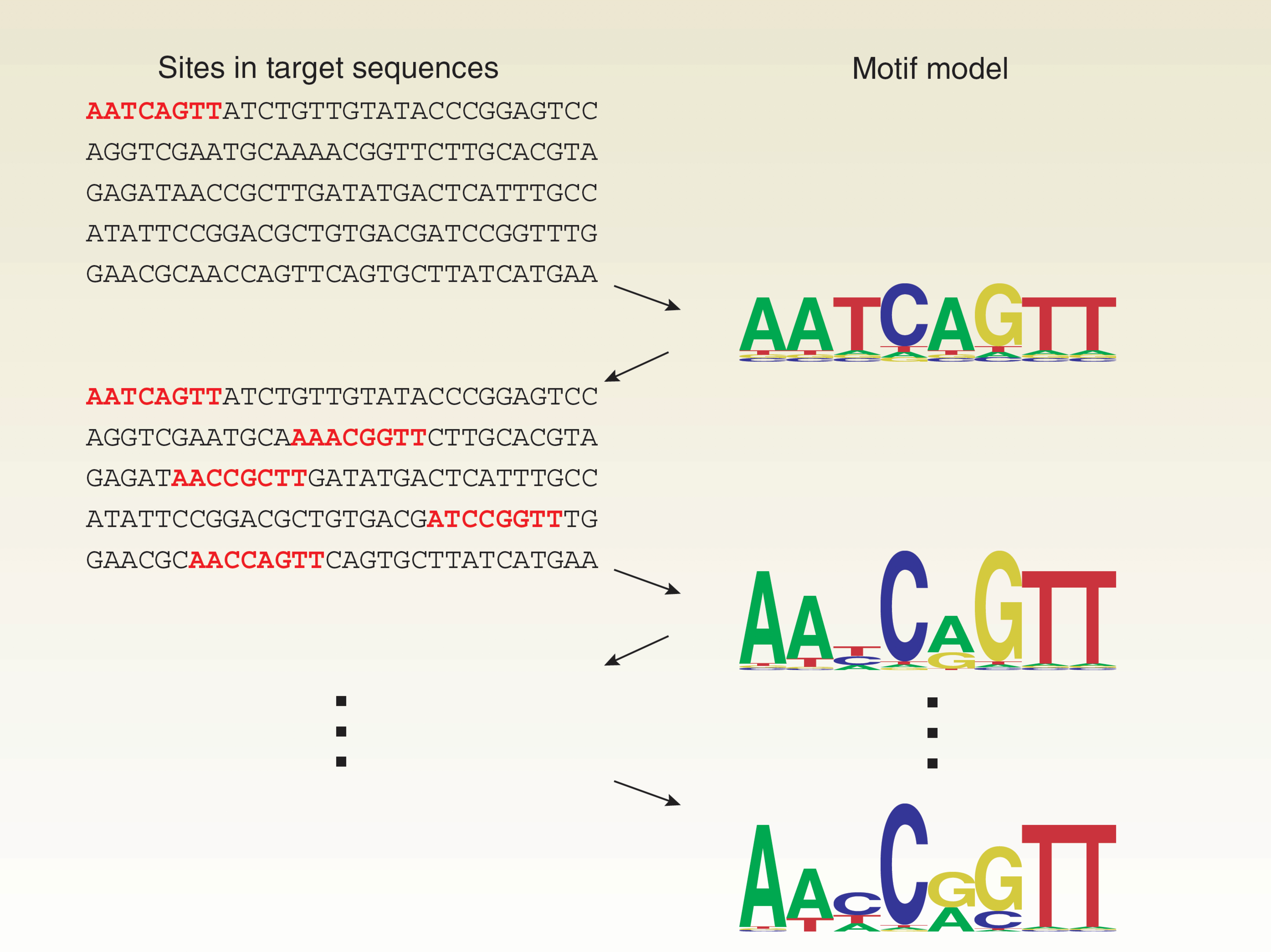
D’haeseleer, Patrik. 2006. “How Does DNA Sequence Motif Discovery Work?”Nature Biotechnology 24 (8): 959–61. https://doi.org/10.1038/nbt0806-959.
Géron, Aurélien. 2022. Hands-on Machine Learning with Scikit-Learn, Keras, and TensorFlow. 3rd ed. O’Reilly Media, Inc.
Goodfellow, Ian, Yoshua Bengio, and Aaron Courville. 2016. Deep Learning. Adaptive Computation and Machine Learning. MIT Press. https://dblp.org/rec/books/daglib/0040158.
Hornik, Kurt, Maxwell Stinchcombe, and Halbert White. 1989. “Multilayer Feedforward Networks Are Universal Approximators.”Neural Networks 2 (5): 359–66. https://doi.org/https://doi.org/10.1016/0893-6080(89)90020-8.
LeNail, Alexander. 2019. “NN-SVG: Publication-Ready Neural Network Architecture Schematics.”Journal of Open Source Software 4 (33): 747. https://doi.org/10.21105/joss.00747.
McCulloch, Warren S, and Walter Pitts. 1943. “A logical calculus of the ideas immanent in nervous activity.”The Bulletin of Mathematical Biophysics 5 (4): 115–33. https://doi.org/10.1007/bf02478259.
Minsky, Marvin, and Seymour Papert. 1969. Perceptrons: An Introduction to Computational Geometry. Cambridge, MA, USA: MIT Press.
Rosenblatt, F. 1958. “The perceptron: A probabilistic model for information storage and organization in the brain.”Psychological Review 65 (6): 386–408. https://doi.org/10.1037/h0042519.
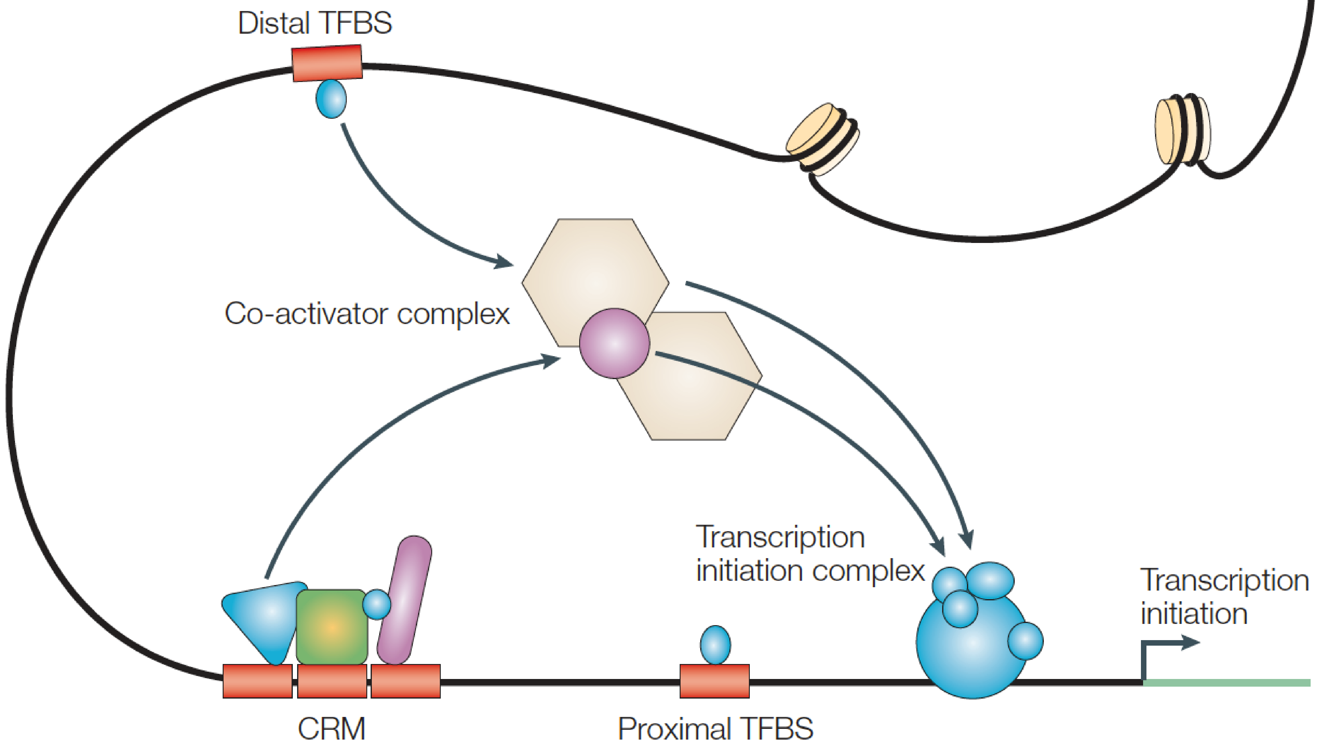
Wasserman, WW, and A Sandelin. 2004. “Applied bioinformatics for the identification of regulatory elements.”Nature Reviews Genetics 5 (4): 276–87. https://doi.org/10.1038/nrg1315.
Zou, James, Mikael Huss, Abubakar Abid, Pejman Mohammadi, Ali Torkamani, and Amalio Telenti. 2019. “A Primer on Deep Learning in Genomics.”Nature Genetics 51 (1): 12–18. https://doi.org/10.1038/s41588-018-0295-5.