In this lecture, we will explore the fundamentals of Convolutional Neural Networks (CNNs) and their role in deep learning. We will begin by discussing the hierarchical structure of deep learning models and the advantages of deep networks over shallow ones. The lecture will cover convolutional operations, including kernels, receptive fields, padding, and stride, and explain their significance in feature extraction. Additionally, we will examine the importance of pooling layers in reducing dimensionality and improving computational efficiency. By the end of the session, students will gain a solid understanding of CNN architectures and their applications in bioinformatics and beyond.
Learning Objectives
Upon completing this lecture, students will be able to:
Explain the hierarchical representation of concepts in deep learning.
Compare deep and shallow neural networks in terms of efficiency and expressiveness.
Describe the structure and function of Convolutional Neural Networks (CNNs).
Understand convolution operations, including kernels and feature extraction.
Explain the concepts of receptive fields, padding, and stride in CNNs.
Discuss the role and benefits of pooling layers in CNN architectures.
Apply CNNs in bioinformatics and recognize their impact on genomic analysis.
Today, we have a particularly dense agenda. The study of convolutional networks involves multiple levels of complexity. Please feel free to ask questions if you need clarification.
Detailed learning objectives.
Explain the Hierarchy of Concepts in Deep Learning
Understand how deep learning models build hierarchical representations of data.
Recognize how this hierarchy reduces the need for manual feature engineering.
Compare Deep and Shallow Neural Networks
Discuss why deep networks are more parameter-efficient than shallow networks.
Explain the benefits of depth in neural network architectures.
Describe the Structure and Function of Convolutional Neural Networks (CNNs)
Understand how CNNs detect local patterns in data.
Explain how convolutional layers reduce the number of parameters through weight sharing.
Understand Convolution Operations Using Kernels
Describe how kernels (filters) are applied over input data to perform convolutions.
Explain how feature maps are generated from convolution operations.
Explain Receptive Fields, Padding, and Stride in CNNs
Define the concept of a receptive field in convolutional layers.
Understand how padding and stride affect the output dimensions and computation.
Discuss the Role and Benefits of Pooling Layers
Explain how pooling layers reduce spatial dimensions and control overfitting.
Describe how pooling introduces translation invariance in CNNs.
Foreword
Convolutional Neural Networks (CNNs) have significantly contributed to the advancement and integration of deep learning technologies.
They are extensively applied in numerous life science domains, as evidenced in research such as Zeng et al. (2016) and He et al. (2020).
CNN architectures are categorized into 1D, 2D, and 3D models.
Although 1D convolutions offer simplicity, this discussion will commence with 2D convolutions due to their prevalent use and to illustrate the conceptual hierarchy inherent in these models.
Introduction
Convolutional Neural Networks
Yann LeCun, recognized as one of the three pioneers of deep learning and the inventor of Convolutional Neural Networks (CNNs), frequently engages in discussions with Elon Musk on the social media platform X (previously known as Twitter).
In the book “Deep Learning” (Goodfellow, Bengio, and Courville 2016), authors Goodfellow, Bengio, and Courville define deep learning as a subset of machine learning that enables computers to “understand the world in terms of a hierarchy of concepts.”
This hierarchical approach is one of deep learning’s most significant contributions. It reduces the need for manual feature engineering and redirects the focus toward the engineering of neural network architectures.
Convolutional Neural Networks (CNNs) have had a profound impact on the field of machine learning, particularly in areas involving image and video processing.
Revolutionizing Image Recognition: CNNs have significantly advanced the state of the art in image recognition and classification, achieving high accuracy across various datasets. This has led to breakthroughs in fields such as medical imaging, autonomous vehicles, and facial recognition.
Feature Extraction: CNNs automatically learn to extract features from raw data, eliminating the need for manual feature engineering. This capability has been crucial in handling complex data patterns and has expanded the applicability of machine learning to diverse domains.
Transfer Learning: CNNs facilitate transfer learning, where pre-trained networks on large datasets can be fine-tuned for specific tasks with limited data. This has made CNNs accessible and effective for a wide range of applications beyond their original training scope.
Advancements in Deep Learning: The success of CNNs has spurred further research in deep learning architectures, inspiring the development of more sophisticated models like recurrent neural networks (RNNs), long short-term memory networks (LSTMs), and transformer models.
Broader Application Areas: Beyond image processing, CNNs have been adapted for natural language processing, audio processing, and even in bioinformatics for tasks such as protein structure prediction and genomics.
Implications for Real-World Applications: CNNs have enabled practical applications in fields such as healthcare, where they assist in diagnostic imaging, and in security, where they enhance surveillance systems. They have also contributed to advancements in virtual reality, gaming, and augmented reality.
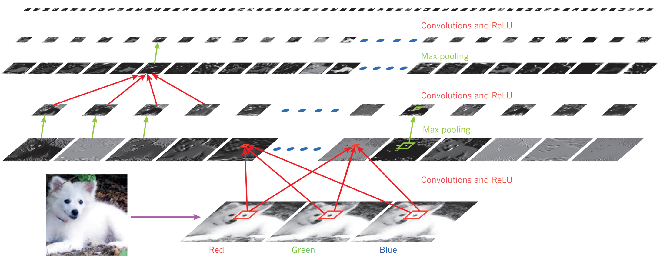
Hierarchy of Concepts
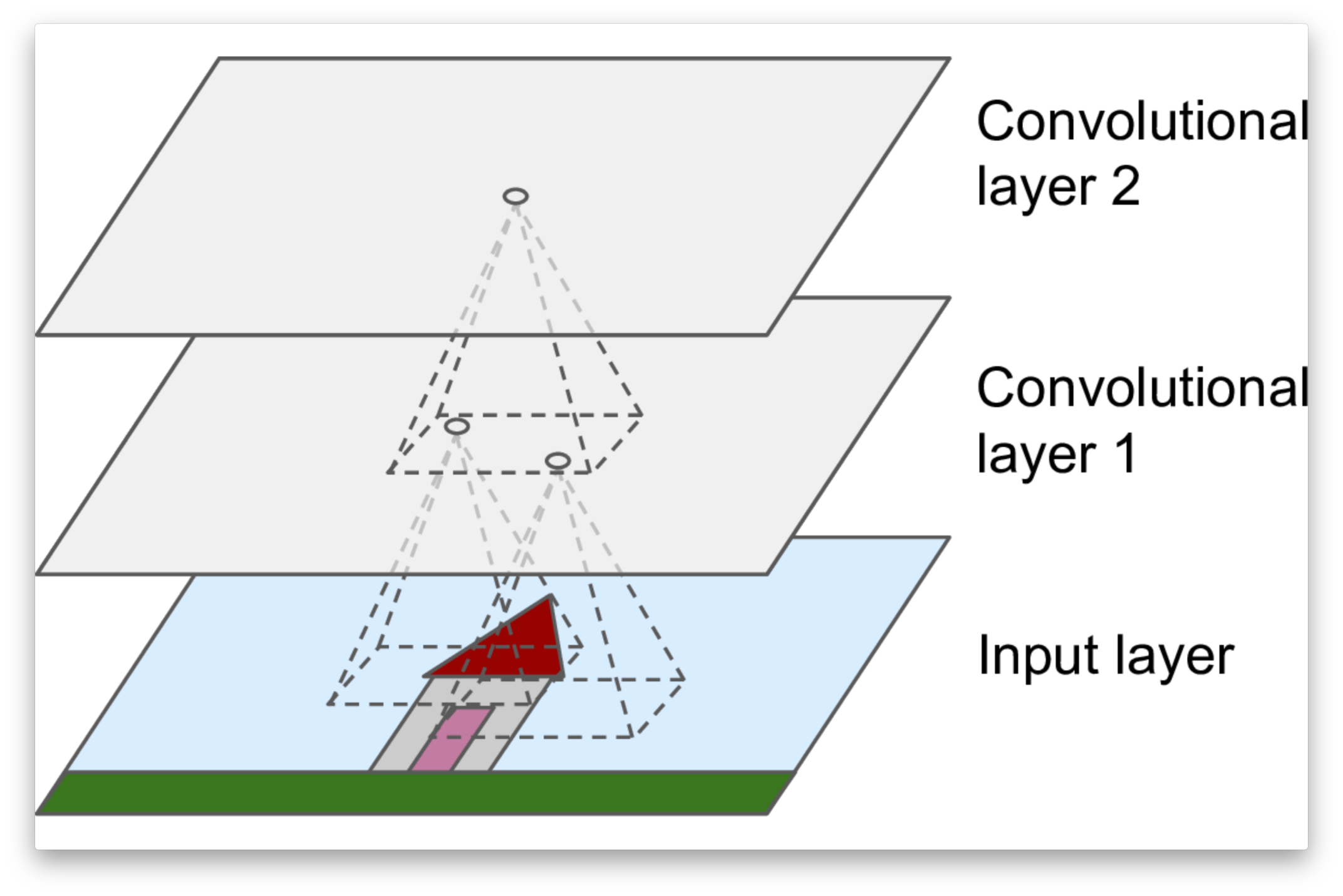
Each layer detects patterns from the output of the layer preceding it.
In other words, proceeding from the input to the output of the network, the network uncovers “patterns of patterns”.
Analyzing an image, the networks first detect simple patterns, such as vertical, horizontal, diagonal lines, arcs, etc.
These are then combined to form corners, crosses, etc.
(This illustrates how transfer learning works and why retaining the bottom layers only.)
But Also …
“An MLP with just one hidden layer can theoretically model even the most complex functions, provided it has enough neurons. But for complex problems, deep networks have a much higher parameter efficiency than shallow ones: they can model complex functions using exponentially fewer neurons than shallow nets, allowing them to reach much better performance with the same amount of training data.”
for \(l=1 \ldots k\). - The number of parameters in grows rapidly:
\[
(\text{size of layer}_{l-1} + 1) \times \text{size of layer}_{l}
\]
Image Classification Task
Consider an RGB image with dimensions \(224 \times 224\), which is relatively small by contemporary benchmarks.
The image consists of \(224 \times 224 \times 3 = 150,528\)input features.
A neural network with merely a single hidden dense layer would require over 22,658,678,784 (22 billion) parameters, highlighting the computational complexity involved.
Unlike dense layers, neurons in a convolutional layer are not fully connected to the preceding layer.
Neurons connect only within their receptive fields (rectangular regions).
Convolutional networks originate from the domain of machine vision, which explains their intrinsic compatibility with grid-structured inputs.
The original publication by Yann Lecun has been cited nearly 35,000 times (Lecun et al. 1998).
Kernel
Kernel
Code
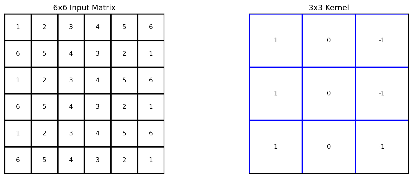
import numpy as npimport matplotlib.pyplot as pltimport matplotlib.patches as patchesdef plot_matrix(ax, matrix, title="Matrix", edge_color='black', face_color='white', highlight_region=None): ax.matshow(matrix, cmap='gray', alpha=0.2)for (i, j), val in np.ndenumerate(matrix): ax.text(j, i, f'{val}', ha='center', va='center', color='black')# Highlight specific region if providedif highlight_region and (i, j) in highlight_region: rect_face_color ='yellow'else: rect_face_color = face_color ax.add_patch(patches.Rectangle((j-0.5, i-0.5), 1, 1, fill=True, edgecolor=edge_color, facecolor=rect_face_color, lw=2)) ax.set_xticks([]) ax.set_yticks([]) ax.set_title(title)def apply_kernel(matrix, kernel): kernel_size = kernel.shape[0] output_size = matrix.shape[0] - kernel_size +1 output = np.zeros((output_size, output_size), dtype=int)for i inrange(output_size):for j inrange(output_size): sub_matrix = matrix[i:i+kernel_size, j:j+kernel_size] output[i, j] = np.sum(sub_matrix * kernel)return output# Define a 6x6 matrix and a 3x3 kernelmatrix = np.array([ [1, 2, 3, 4, 5, 6], [6, 5, 4, 3, 2, 1], [1, 2, 3, 4, 5, 6], [6, 5, 4, 3, 2, 1], [1, 2, 3, 4, 5, 6], [6, 5, 4, 3, 2, 1]])kernel = np.array([ [1, 0, -1], [1, 0, -1], [1, 0, -1]])# Apply the kernel to the matrixoutput = apply_kernel(matrix, kernel)# Plot the original matrix, kernel, and the resultfig, axes = plt.subplots(1, 2, figsize=(12, 4))plot_matrix(axes[0], matrix, "6x6 Input Matrix")plot_matrix(axes[1], kernel, "3x3 Kernel", edge_color='blue')# plot_matrix(axes[2], output, "Output Matrix", edge_color='green')plt.tight_layout()plt.show()
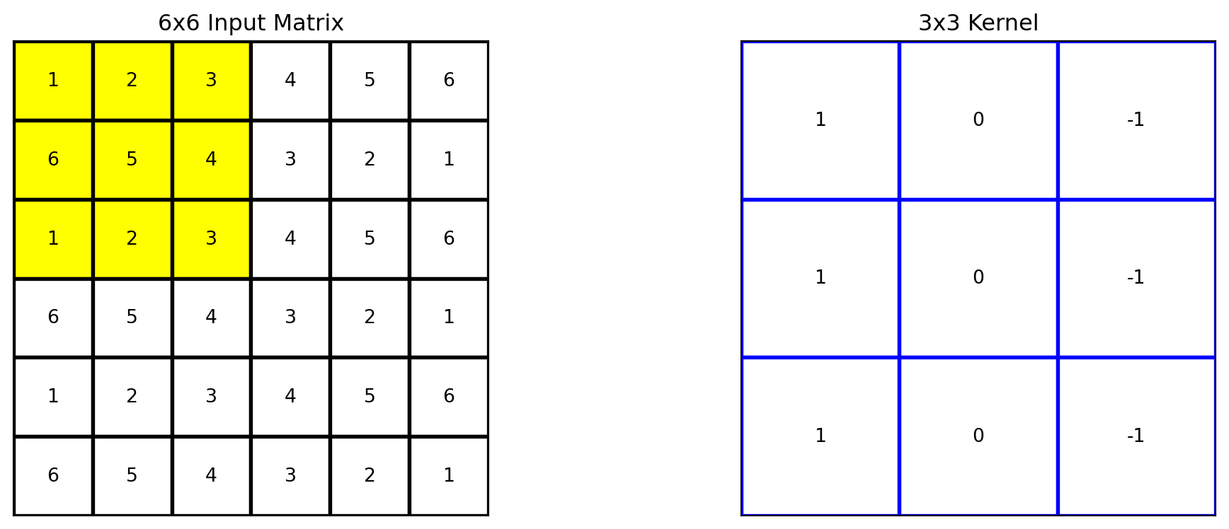
A kernel is a small matrix, usually \(3 \times 3\), \(5 \times 5\), or similar in size, that slides over the input data (such as an image) to perform convolution.
Firstly, we will examine the technical components of convolution, focusing on the interaction between the input matrix and the kernel. Subsequently, we will explore the computational process involved in performing a convolution. Lastly, we will analyze the significance and implications of convolution.
Kernel
Code
# Apply the kernel to the matrixoutput = apply_kernel(matrix, kernel)# Define the region to highlight (top-left 3x3 cells)highlight_region = [(i, j) for i inrange(3) for j inrange(3)]# Plot the original matrix, kernel, and the resultfig, axes = plt.subplots(1, 2, figsize=(12, 4))plot_matrix(axes[0], matrix, "6x6 Input Matrix", highlight_region=highlight_region)plot_matrix(axes[1], kernel, "3x3 Kernel", edge_color='blue')plt.tight_layout()plt.show()
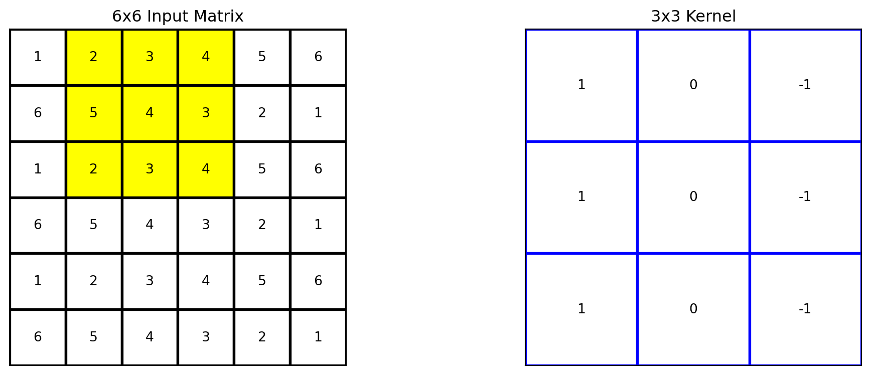
Beginning with the kernel positioned to overlap the upper-left corner of the input matrix.
Kernel
Code
# Apply the kernel to the matrixoutput = apply_kernel(matrix, kernel)# Define the region to highlight (top-left 3x3 cells)highlight_region = [(i, j) for i inrange(3) for j inrange(1,4)]# Plot the original matrix, kernel, and the resultfig, axes = plt.subplots(1, 2, figsize=(12, 4))plot_matrix(axes[0], matrix, "6x6 Input Matrix", highlight_region=highlight_region)plot_matrix(axes[1], kernel, "3x3 Kernel", edge_color='blue')plt.tight_layout()plt.show()
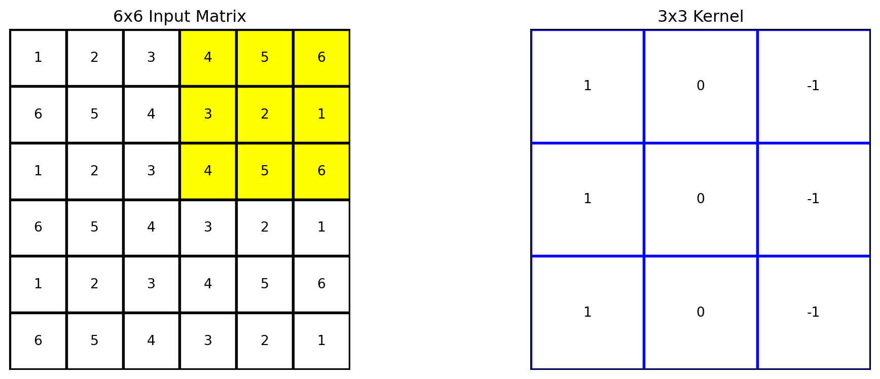
It can be moved to the right three times.
Kernel
Code
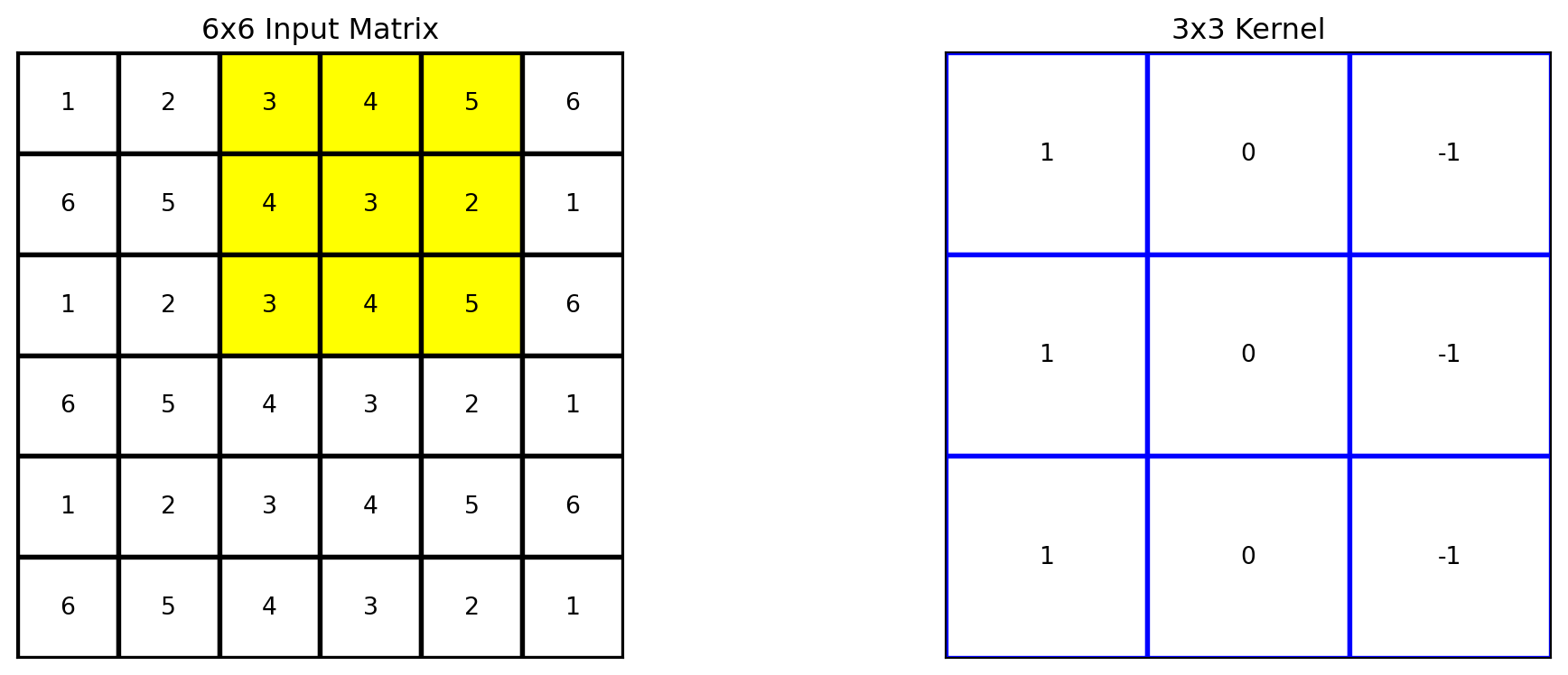
# Apply the kernel to the matrixoutput = apply_kernel(matrix, kernel)# Define the region to highlight (top-left 3x3 cells)highlight_region = [(i, j) for i inrange(3) for j inrange(2,5)]# Plot the original matrix, kernel, and the resultfig, axes = plt.subplots(1, 2, figsize=(12, 4))plot_matrix(axes[0], matrix, "6x6 Input Matrix", highlight_region=highlight_region)plot_matrix(axes[1], kernel, "3x3 Kernel", edge_color='blue')plt.tight_layout()plt.show()
Kernel
Code
# Apply the kernel to the matrixoutput = apply_kernel(matrix, kernel)# Define the region to highlight (top-left 3x3 cells)highlight_region = [(i, j) for i inrange(3) for j inrange(3,6)]# Plot the original matrix, kernel, and the resultfig, axes = plt.subplots(1, 2, figsize=(12, 4))plot_matrix(axes[0], matrix, "6x6 Input Matrix", highlight_region=highlight_region)plot_matrix(axes[1], kernel, "3x3 Kernel", edge_color='blue')plt.tight_layout()plt.show()
Kernel
Code
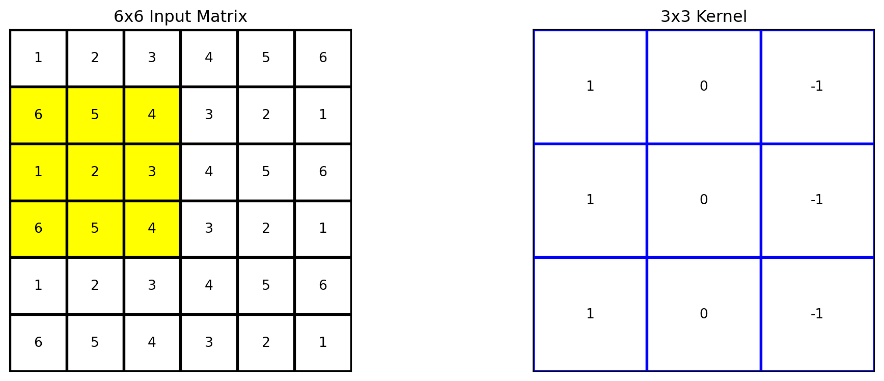
# Apply the kernel to the matrixoutput = apply_kernel(matrix, kernel)# Define the region to highlight (top-left 3x3 cells)highlight_region = [(i, j) for i inrange(1,4) for j inrange(3)]# Plot the original matrix, kernel, and the resultfig, axes = plt.subplots(1, 2, figsize=(12, 4))plot_matrix(axes[0], matrix, "6x6 Input Matrix", highlight_region=highlight_region)plot_matrix(axes[1], kernel, "3x3 Kernel", edge_color='blue')plt.tight_layout()plt.show()
The kernel can then be moved to the second row of the input matrix, and moved to the right three times.
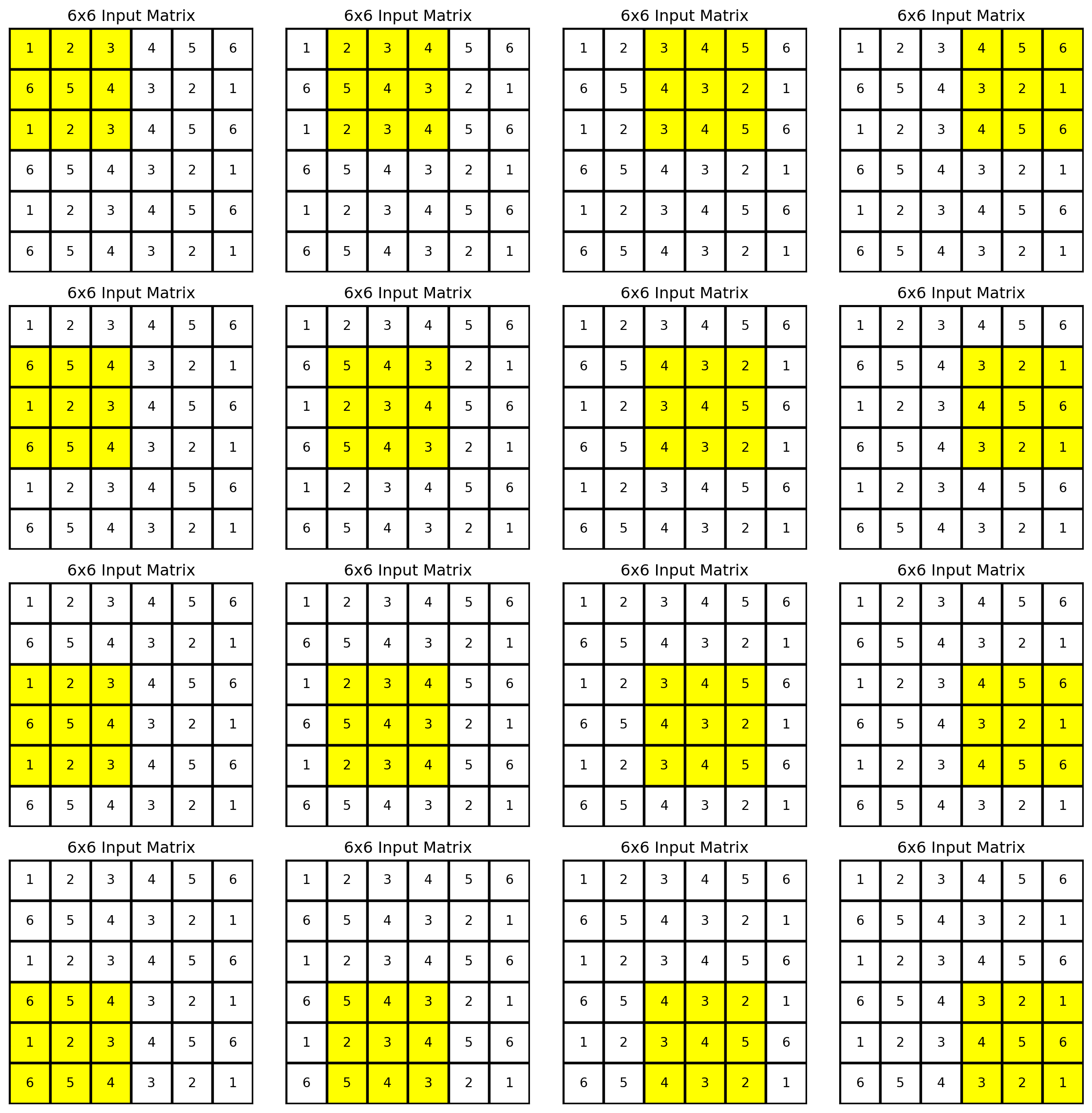
How many placements of the kernel over the input matrix are there? \(4 \times 4 = 16\).
Kernel Placements
Code
# Apply the kernel to the matrixoutput = apply_kernel(matrix, kernel)fig, axes = plt.subplots(4, 4, figsize=(12, 12))for row inrange(4):for col inrange(4):# Define the region to highlight (top-left 3x3 cells) highlight_region = [(i, j) for i inrange(row, row+3) for j inrange(col, col+3)]# Plot the original matrix, kernel, and the result plot_matrix(axes[row,col], matrix, "6x6 Input Matrix", highlight_region=highlight_region)plt.tight_layout()plt.show()
Kernel
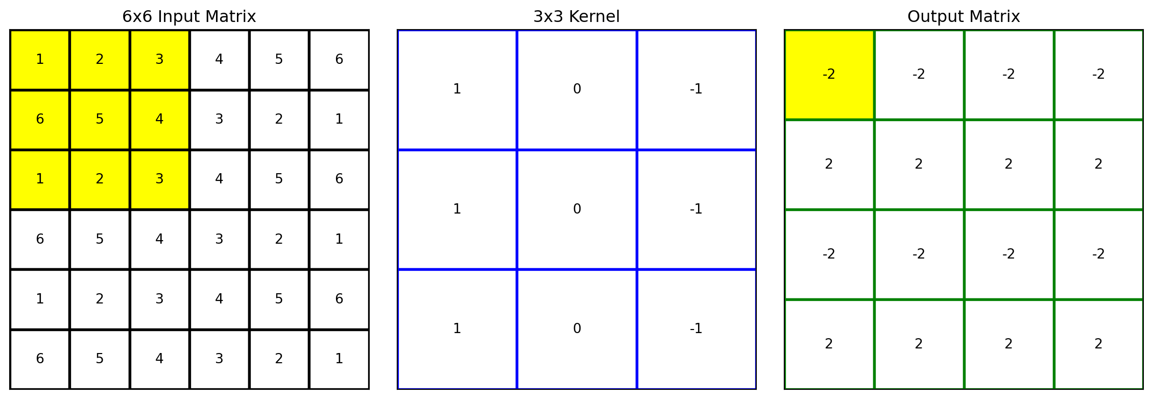
With the kernel placed over a specific region of the input matrix, the convolution is element-wise multiplication (each element of the kernel is multiplied by the corresponding element of the input matrix region it overlaps) followed by a summation of the results to produce a single scalar value.
Kernel
Code
# Apply the kernel to the matrixoutput = apply_kernel(matrix, kernel)# Define the region to highlight (top-left 3x3 cells)highlight_region = [(i, j) for i inrange(3) for j inrange(3)]# Plot the original matrix, kernel, and the resultfig, axes = plt.subplots(1, 2, figsize=(12, 4))plot_matrix(axes[0], matrix, "6x6 Input Matrix", highlight_region=highlight_region)plot_matrix(axes[1], kernel, "3x3 Kernel", edge_color='blue')plt.tight_layout()plt.show()
The 16 resulting values can be organized into an output matrix. The element at position (0,0) in this output matrix represents the result of applying the convolution operation with the kernel at the initial position on the input matrix. In convolutional neural networks, the output matrix is referred to as a feature map.
It is referred to as a feature map because these outputs serve as features for the subsequent layer. In CNNs, the term “feature map” refers to the output of a convolutional layer after applying filters to the input data. These feature maps capture various patterns or features from the input, such as edges or textures in image data.
The output feature maps of one layer become the input for the next layer, effectively serving as features that the subsequent layer can use to learn more complex patterns. This hierarchical feature extraction process is a key characteristic of CNNs, allowing them to build progressively more abstract and high-level representations of the input data as the network depth increases.
Blurring
Code
import numpy as npfrom PIL import Imageimport matplotlib.pyplot as pltfrom scipy.ndimage import convolvedef apply_kernel_to_image(image_path, kernel):# Load the image and convert it to grayscale image = Image.open(image_path).convert('L') image_array = np.array(image)# Apply the convolution using the provided kernel convolved_array = convolve(image_array, kernel, mode='reflect')# Convert the convolved array back to an image convolved_image = Image.fromarray(convolved_array)# Display the original and convolved images plt.figure(figsize=(10, 4)) plt.subplot(1, 2, 1) plt.title('Original Image') plt.imshow(image_array, cmap='gray') plt.axis('off') plt.subplot(1, 2, 2) plt.title('Convolved Image') plt.imshow(convolved_image, cmap='gray') plt.axis('off') plt.tight_layout() plt.show()# Define the 7x7 averaging kernelkernel = np.array([ [1/49, 1/49, 1/49, 1/49, 1/49, 1/49, 1/49], [1/49, 1/49, 1/49, 1/49, 1/49, 1/49, 1/49], [1/49, 1/49, 1/49, 1/49, 1/49, 1/49, 1/49], [1/49, 1/49, 1/49, 1/49, 1/49, 1/49, 1/49], [1/49, 1/49, 1/49, 1/49, 1/49, 1/49, 1/49], [1/49, 1/49, 1/49, 1/49, 1/49, 1/49, 1/49], [1/49, 1/49, 1/49, 1/49, 1/49, 1/49, 1/49]])# Apply the kernel to the image (provide your image path here)image_path ='../../assets/images/uottawa_hor_black.png'apply_kernel_to_image(image_path, kernel)
A pixel is transformed into the average of itself and its eight surrounding neighbors, resulting in a blurred effect on the image.
The application of kernels to images has been a longstanding practice in the field of image processing.
Vertical Edge detection
Code
# Define the 3x3 vertical edge detection kernelkernel = np.array([ [-1, 0, 1], [-2, 0, 2], [-1, 0, 1]])# Apply the kernel to the image (provide your image path here)image_path ='../../assets/images/uottawa_hor_black.png'apply_kernel_to_image(image_path, kernel)
This kernel detects vertical edges by emphasizing differences in intensity between adjacent columns. It subtracts pixel values on the left from those on the right, enhancing vertical transitions and suppressing uniform regions.
This is a type of edge detection kernel, specifically a horizontal gradient filter or a Sobel operator. It’s designed to detect changes in intensity along the horizontal axis, emphasizing vertical edges in an image.
When this kernel is convolved with an image:
It highlights vertical edges by calculating the difference in pixel intensity between the left and right sides of a point.
The negative values (-1) on the left subtract intensity, while the positive values (1) on the right add intensity, effectively measuring the horizontal gradient.
The zeros in the middle ignore the central pixel’s contribution, focusing only on the contrast between left and right neighbors.
The result is an image where:
Vertical edges (e.g., the boundary between a dark object and a light background) appear bright or dark, depending on the direction of the intensity change.
Horizontal edges or uniform areas tend to be suppressed (close to zero).
Imagine sliding this kernel over an image like a scanner. For each pixel:
It looks at the pixels to its left (subtracting their value with -1) and to its right (adding their value with 1).
If the left and right sides are similar (e.g., same color), the result is near zero (no edge).
If the left is dark and the right is light (or vice versa), the result is a strong positive or negative value, showing a vertical edge.
This is useful in computer vision (like in Tesla’s CNNs) to help detect object boundaries or lane lines by emphasizing where pixel values change sharply in the horizontal direction.
Horizontal Edge detection
Code
# Define the 3x3 horizontal edge detection kernelkernel = np.array([ [1, 2, 1], # Top row (positive) [0, 0, 0], # Middle row (neutral) [-1, -2, -1] # Bottom row (negative)])# Apply the kernel to the image (provide your image path here)image_path ='../../assets/images/uottawa_hor_black.png'apply_kernel_to_image(image_path, kernel)
This kernel detects horizontal edges by highlighting differences in intensity between adjacent rows. It subtracts pixel values in the upper row from those in the lower row, accentuating horizontal transitions while minimizing uniform areas.
Kernels
In contrast to image processing, where kernels are manually defined by the user, in convolutional networks, the kernels are automatically learned by the network.
Each unit is connected to neurons in its receptive fields.
Unit \(i,j\) in layer \(l\) is connected to the units \(i\) to \(i+f_h-1\), \(j\) to \(j+f_w-1\) of the layer \(l-1\), where \(f_h\) and \(f_w\) are respectively the height and width of the receptive field.
Padding
Zero padding. In order to have layers of the same size, the grid can be padded with zeros.
Stride. It is possible to connect a larger layer \((l-1)\) to a smaller one \((l)\) by skipping units. The number of units skipped is called stride, \(s_h\) and \(s_w\).
. . .
Unit \(i,j\) in layer \(l\) is connected to the units \(i \times s_h\) to \(i \times s_h + f_h - 1\), \(j \times s_w\) to \(j \times s_w + f_w - 1\) of the layer \(l-1\), where \(f_h\) and \(f_w\) are respectively the height and width of the receptive field, \(s_h\) and \(s_w\) are respectively the height and widthstrides.
A window of size \(f_h \times f_w\) is moved over the output of layers \(l-1\), referred to as the input feature map, position by position.
For each location, the product is calculated between the extracted patch and a matrix of the same size, known as a convolution kernel or filter. The sum of the values in the resulting matrix constitutes the output for that location.
“Thus, a layer full of neurons using the same filter outputs a feature map.”
“Of course, you do not have to define the filters manually: instead, during training the convolutional layer will automatically learn the most useful filters for its task.”
Feature Map: In convolutional neural networks (CNNs), the output of a convolution operation is known as a feature map. It captures the features of the input data as processed by a specific kernel.
Summmary
Kernel Parameters: The parameters of the kernel are learned through the backpropagation process, allowing the network to optimize its feature extraction capabilities based on the training data.
Summmary
Bias Term: A single bias term is added uniformly to all entries of the feature map. This bias helps adjust the activation level, providing additional flexibility for the network to better fit the data.
Summmary
Activation Function: Following the addition of the bias, the feature map values are typically passed through an activation function, such as ReLU (Rectified Linear Unit). The ReLU function introduces non-linearity by setting negative values to zero while retaining positive values, enabling the network to learn more complex patterns.
Pooling
Pooling
A pooling layer exhibits similarities to a convolutional layer.
Each neuron in a pooling layer is connected to a set of neurons within a receptive field.
However, unlike convolutional layers, pooling layers do not possess weights.
Instead, they produce an output by applying an aggregating function, commonly max or mean.
Similar to convolutional layers, pooling layers allow specification of the receptive field size, padding, and stride. For the MaxPool2D function, the default receptive field size is \(2 \times 2\).
In a pooling layer, specifically max pooling, the max function is inherently nondifferentiable because it involves selecting the maximum value from a set of inputs. However, in the context of backpropagation in neural networks, we can work around this by using a concept known as the “gradient of the max function.”
Here’s how it is done:
Forward Pass: During the forward pass, the max pooling layer selects the maximum value from each pooling region (e.g., a 2x2 window) and passes these values to the next layer.
Backward Pass: During backpropagation, the gradient is propagated only to the input that was the maximum value in the forward pass. This means that the derivative is 1 for the position that held the maximum value and 0 for all other positions within the pooling window.
This approach effectively allows the max operation to participate in gradient-based optimization processes like backpropagation, even though the max function itself is nondifferentiable. By assigning the gradient to the position of the maximum value, the network can learn which features are most important for the task at hand.
Pooling
This subsampling process leads to a reduction in network size; each window of dimensions \(f_h \times f_w\) is condensed to a single value, typically the maximum or mean of that window.
A max pooling layer provides a degree of invariance to small translations (Géron (2019), § 14).
Pooling
Dimensionality Reduction: Pooling layers reduce the spatial dimensions (width and height) of the input feature maps. This reduction decreases the number of parameters and computational load in the network, which can help prevent overfitting.
Pooling
Feature Extraction: By summarizing the presence of features in a region, pooling layers help retain the most critical information while discarding less important details. This process enables the network to focus on the most salient features.
Pooling
Translation Invariance: Pooling introduces a degree of invariance to translations and distortions in the input. For instance, max pooling captures the most prominent feature in a local region, making the network less sensitive to small shifts or variations in the input.
Pooling
Noise Reduction: Pooling can help smooth out noise in the input by aggregating information over a region, thus emphasizing consistent features over random variations.
Pooling
Hierarchical Feature Learning: By reducing the spatial dimensions progressively through the layers, pooling layers allow the network to build a hierarchical representation of the input data, capturing increasingly abstract and complex features at deeper layers.
/Users/turcotte/opt/micromamba/envs/ml4bio/lib/python3.10/site-packages/keras/src/layers/convolutional/base_conv.py:107: UserWarning:

Do not pass an `input_shape`/`input_dim` argument to a layer. When using Sequential models, prefer using an `Input(shape)` object as the first layer in the model instead.
Géron (2022) Chapter 11, test accuracy of 92% on the Fashion-MNIST dataset
The previously discussed model, which comprised fully connected (Dense) layers, attained a test accuracy of 88%.
We will look at pooling next.
Convolutional Neural Networks
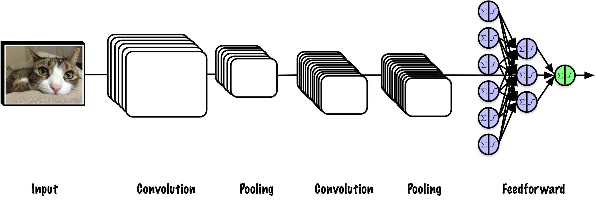
The architecture involves sequentially stacking several convolutional layers, each followed by a ReLU activation layer, and then a pooling layer. As this process continues, the spatial dimensions of the image representation decrease. Concurrently, the number of feature maps increases, as illustrated in our Keras example. At the top of this stack, a standard feedforward neural network is incorporated.
AlexNet consists of eight layers with learnable parameters: five convolutional layers followed by three fully connected layers. The architecture also includes max-pooling layers, ReLU activation functions, and dropout to improve training performance and reduce overfitting.
Convolutional networks (ConvNets) currently set the state of the art in visual recognition. The aim of this project is to investigate how the ConvNet depth affects their accuracy in the large-scale image recognition setting.
Our main contribution is a rigorous evaluation of networks of increasing depth, which shows that a significant improvement on the prior-art configurations can be achieved by increasing the depth to 16-19 weight layers, which is substantially deeper than what has been used in the prior art. To reduce the number of parameters in such very deep networks, we use very small 3×3 filters in all convolutional layers (the convolution stride is set to 1). Please see our publication for more details.
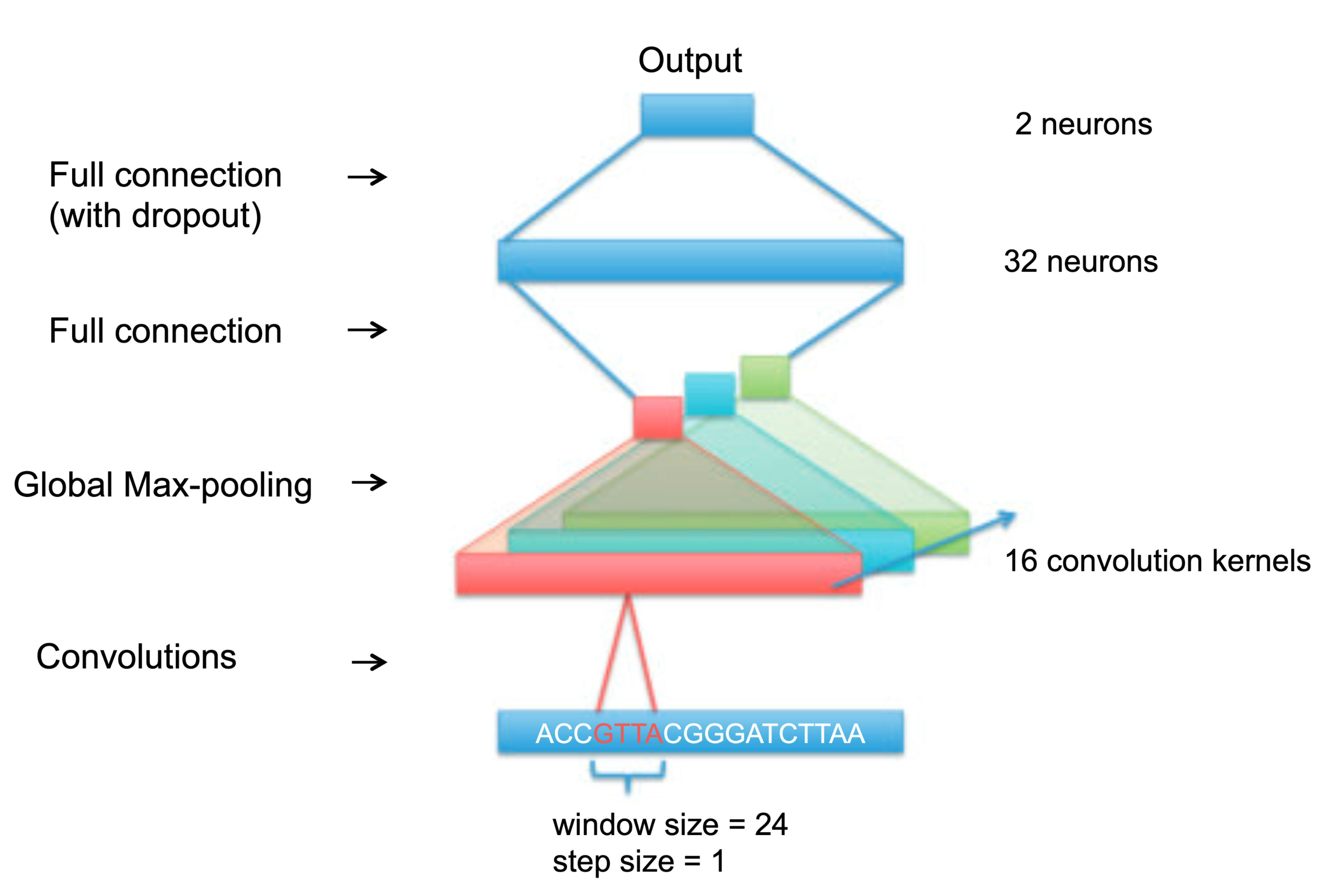
This study examines nine architectural variants of neural networks by altering their width, depth, and pooling configurations. The networks’ performance is assessed across 690 distinct ChIP-seq experiments.
Conclusion: “We found for both tasks, classification performance increases with the number of convolution kernels, and the use of local pooling or more convolutional layers has little, if not negative, effect on the performance”
import numpy as npimport pandas as pdimport matplotlib.pyplot as pltimport seaborn as snsimport requestsfrom sklearn.preprocessing import LabelEncoder, OneHotEncodernp.set_printoptions(threshold=40)# Define the base URL for accessing genomic sequence dataBASE_URL ='https://raw.githubusercontent.com/abidlabs/deep-learning-genomics-primer/master/'SEQUENCES_URL = BASE_URL +'sequences.txt'
try:# Fetch the sequences from the URL response = requests.get(SEQUENCES_URL) response.raise_for_status() # Raise an error if the request was unsuccessful# Split the text data into a list of sequences, removing any empty lines sequences = response.text.split('\n') sequences =list(filter(None, sequences)) # Removes empty strings from the list# Convert sequences into a pandas DataFrame for easy viewing df = pd.DataFrame(sequences, index=np.arange(1, len(sequences) +1), columns=['Sequences'])# Display the first few rows of the datasetprint(df.head())except requests.RequestException as e:print(f"Error fetching sequences: {e}")
/Users/turcotte/opt/micromamba/envs/ml4bio/lib/python3.10/site-packages/keras/src/layers/convolutional/base_conv.py:107: UserWarning:

Do not pass an `input_shape`/`input_dim` argument to a layer. When using Sequential models, prefer using an `Input(shape)` object as the first layer in the model instead.
It begins with fundamental principles and extends to contemporary topics such as transformers, diffusion models, graph neural networks, autoencoders, adversarial networks, and reinforcement learning.
The textbook aims to help readers comprehend these concepts without delving excessively into theoretical details.
It includes sixty-eight Python notebook exercises.
The book follows a “read-first, pay-later” model.
Resources
A guide to convolution arithmetic for deep learning
Consens, Micaela E., Cameron Dufault, Michael Wainberg, Duncan Forster, Mehran Karimzadeh, Hani Goodarzi, Fabian J. Theis, Alan Moses, and Bo Wang. 2025. “Transformers and genome language models.”Nature Machine Intelligence, 1–17. https://doi.org/10.1038/s42256-025-01007-9.
Géron, Aurélien. 2019. Hands-on Machine Learning with Scikit-Learn, Keras, and TensorFlow. 2nd ed. O’Reilly Media.
———. 2022. Hands-on Machine Learning with Scikit-Learn, Keras, and TensorFlow. 3rd ed. O’Reilly Media, Inc.
Goodfellow, Ian, Yoshua Bengio, and Aaron Courville. 2016. Deep Learning. Adaptive Computation and Machine Learning. MIT Press. https://dblp.org/rec/books/daglib/0040158.
He, Ying, Zhen Shen, Qinhu Zhang, Siguo Wang, and De-Shuang Huang. 2020. “A survey on deep learning in DNA/RNA motif mining.”Briefings in Bioinformatics 22 (4): bbaa229. https://doi.org/10.1093/bib/bbaa229.
Lecun, Y., L. Bottou, Y. Bengio, and P. Haffner. 1998. “Gradient-Based Learning Applied to Document Recognition.”Proceedings of the IEEE 86 (11): 2278–2324. https://doi.org/10.1109/5.726791.
Prince, Simon J. D. 2023. Understanding Deep Learning. The MIT Press. http://udlbook.com.
Simonyan, Karen, and Andrew Zisserman. 2015. “Very Deep Convolutional Networks for Large-Scale Image Recognition.” In International Conference on Learning Representations.
Zeng, Haoyang, Matthew D Edwards, Ge Liu, and David K Gifford. 2016. “Convolutional Neural Network Architectures for Predicting DNA-Protein Binding.”Bioinformatics (Oxford, England) 32 (12): i121–27. https://doi.org/10.1093/bioinformatics/btw255.
Zou, James, Mikael Huss, Abubakar Abid, Pejman Mohammadi, Ali Torkamani, and Amalio Telenti. 2019. “A Primer on Deep Learning in Genomics.”Nature Genetics 51 (1): 12–18. https://doi.org/10.1038/s41588-018-0295-5.