School of Electrical Engineering and Computer Science
University of Ottawa
Published
October 13, 2026
This self-study notebook extends Lecture 11’s discussion of nonlinear decision boundaries. We compare two ways to obtain a useful representation: designing features for logistic regression and learning hidden representations with a neural network. It complements the circle dataset in TensorFlow Playground.
The Keras examples can be explored now; the training methods, losses, and regularization techniques are developed in Lectures 12–14.
Data
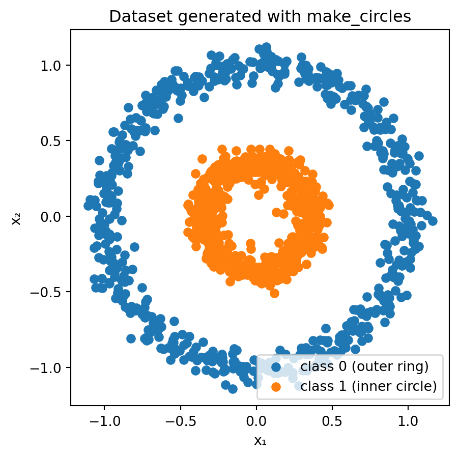
The inner circle is class 1, and the outer ring is class 0. No straight line can separate these two classes in the original input plane.
Logistic regression using only x_1 and x_2 has a straight decision boundary, so it cannot separate the inner circle from the surrounding ring. Logistic regression can nevertheless produce a nonlinear boundary in the input plane if we give it nonlinear features.
TensorFlow Playground offers x_1^2 and x_2^2 as additional features. A network with no hidden layers and one sigmoid output is logistic regression on the selected features. Keeping the two original inputs and both squared inputs gives four features; selecting only the squared inputs gives two.
For a simpler visualization, combine the squared inputs into one feature:
r = x_1^2 + x_2^2.
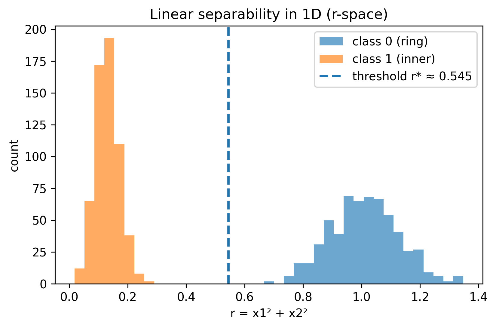
Here, r denotes the squared distance from the origin, rather than the radius itself. Inner-circle points have small r; outer-ring points have large r. Squaring the distance preserves their ordering, so computing a square root is unnecessary.
For the sample generated above, the two bands are separated in r-space. A threshold r^* can separate the classes:
\text{inner if } r < r^*, \qquad \text{outer if } r > r^*.
The same threshold corresponds to a circle in the original input plane. With more noise, the radial bands may overlap, and perfect separation may no longer be possible.
Fit a model in r-space
All models for a dataset use the same split: 60% training, 20% validation, and 20% test. Only training examples are used to fit the parameters. The neural network uses validation loss for early stopping; the test examples are reserved for the final comparison.
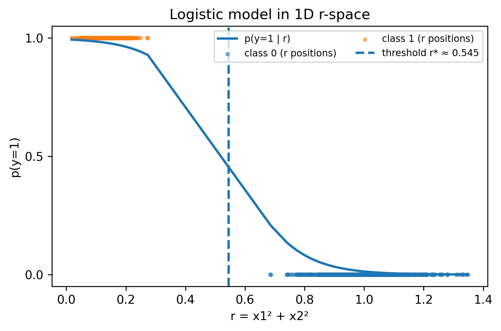
The radial model estimates p(y=1\mid r)=\sigma(wr+b). Its decision boundary is where wr+b=0, or r^*=-b/w. The learned weight is negative because class 1 occupies the smaller radii.
3D view
Lifting each point to (x_1,x_2,r) makes the decision boundary a horizontal plane. Rotate the interactive view to see how the plane separates the two bands.
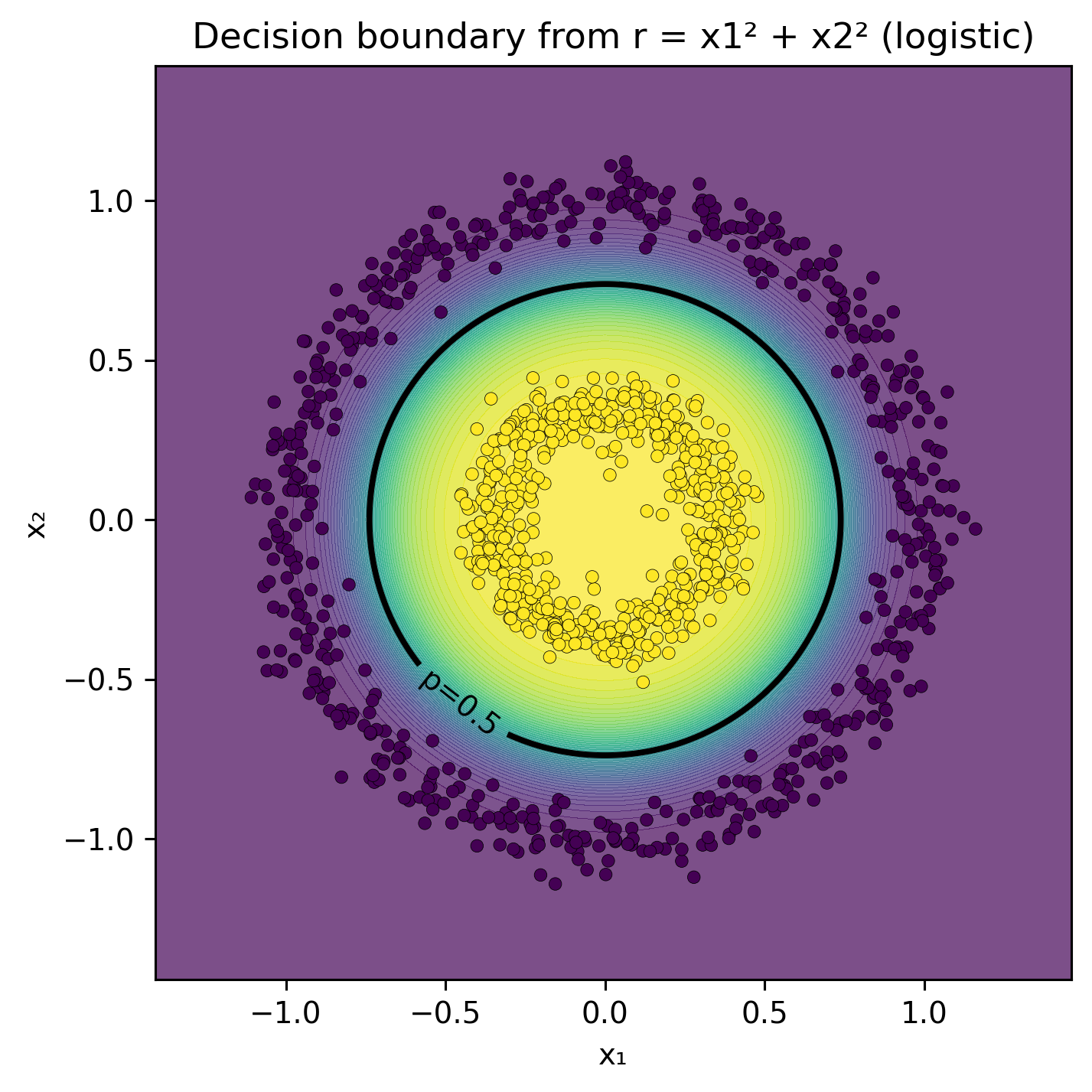
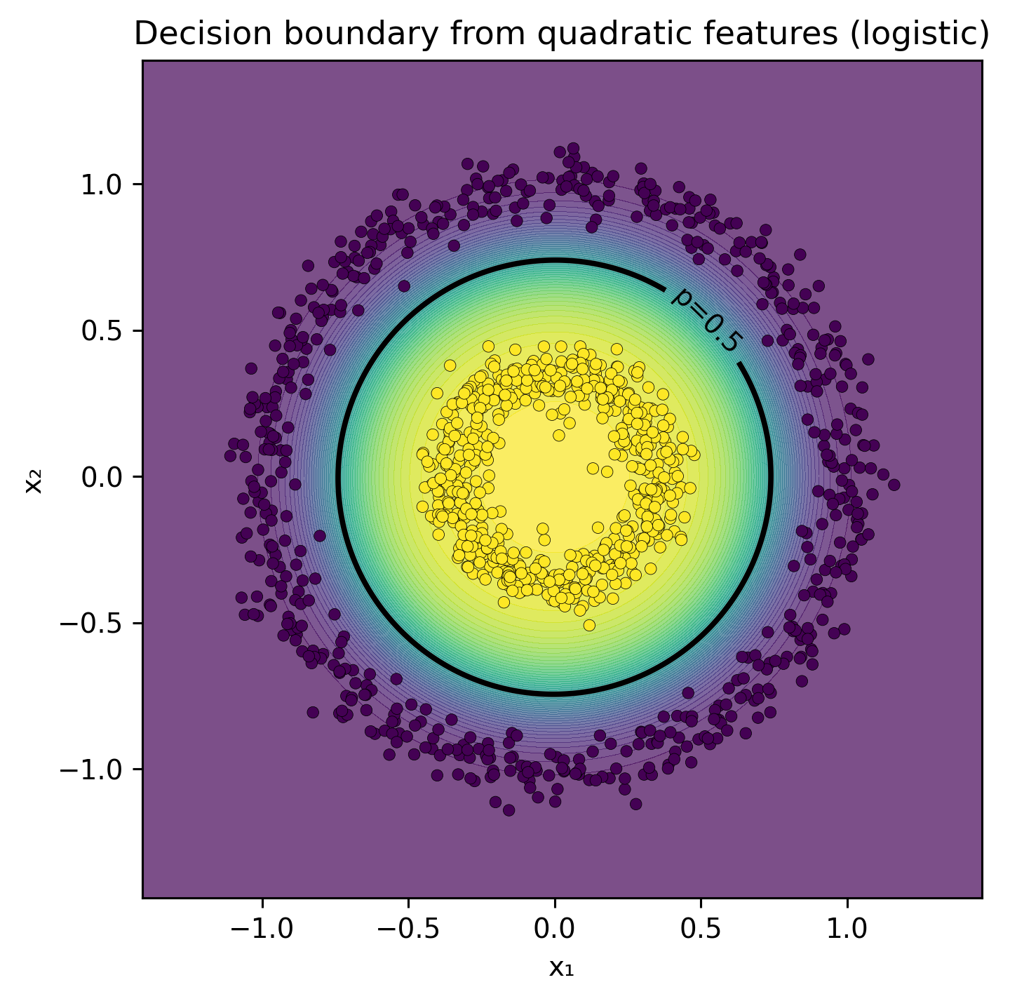
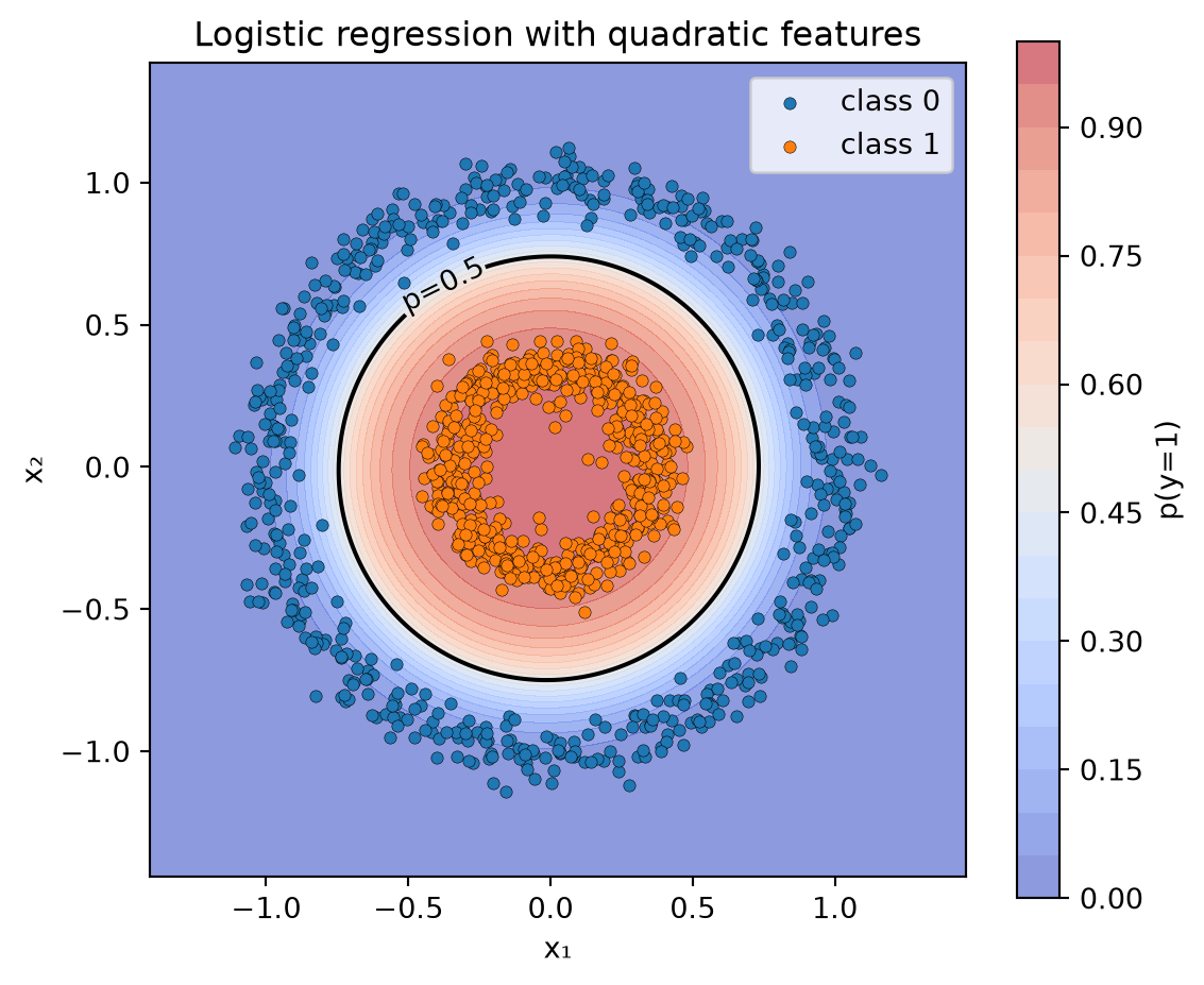
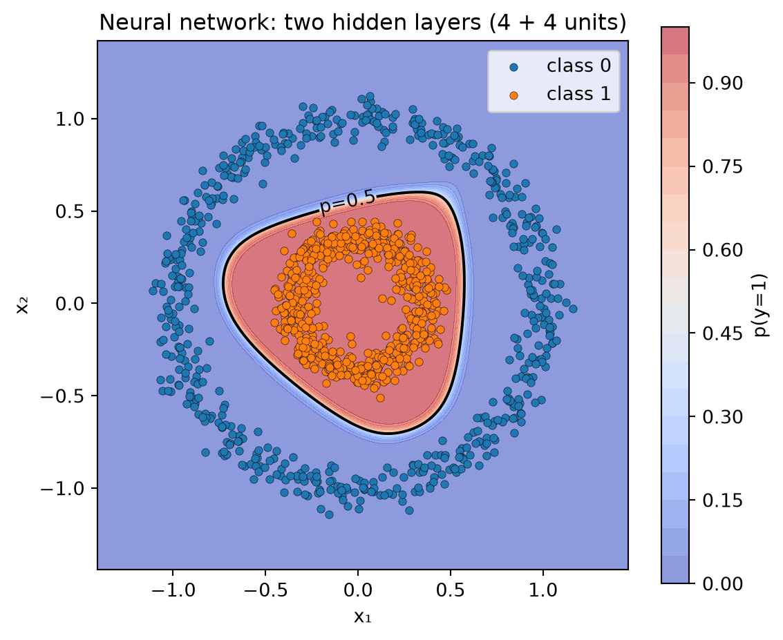
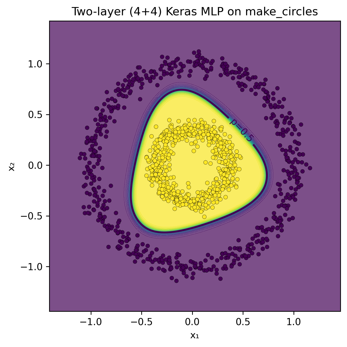
The plotting helpers below will also be used for the quadratic model and the neural networks. Shading shows the estimated probability of class 1; the black contour marks p=0.5. The points show the full generated dataset, while model fitting uses only the training split.
The radial model constrains the squared inputs to share one coefficient, because wr=w(x_1^2+x_2^2). The quadratic model can weight all five features independently. Both can separate these circles, but their fitted boundaries and probabilities need not be identical. Their default regularization also acts on different parameterizations.
The neural network receives only the original inputs x_1 and x_2. It has two hidden layers, each with four units, followed by one sigmoid output: three layers with trainable parameters. The hidden layers use tanh, a nonlinear activation, and learn a representation from the training examples.
This is one working configuration, rather than a claim that tanh always trains faster or better than other activations. Training success depends on the data, initialization, architecture, and optimization settings.
Early stopping monitors validation loss and restores the weights from the epoch with the lowest validation loss. This epoch need not have the highest validation accuracy. We therefore evaluate the restored model directly, rather than taking unrelated values from the training history. See the Keras documentation for the callback’s parameters.
The comparison uses the same held-out examples for every model. It illustrates the effect of representation on this dataset; a successful run does not guarantee the same results for other datasets or training settings.
_, circle_test_accuracy = circle_mlp.evaluate(X_test, y_test, verbose=0)circle_scores = {"Logistic: original inputs": clf_raw.score(X_test, y_test),"Logistic: radial feature": clf_r.score(radial_features(X_test), y_test),"Logistic: quadratic features": quad.score(X_test, y_test),"Neural network: original inputs": circle_test_accuracy,}for name, accuracy in circle_scores.items():print(f"{name:<34} test accuracy = {accuracy:.3f}")
Logistic: original inputs          test accuracy = 0.471
Logistic: radial feature           test accuracy = 1.000
Logistic: quadratic features       test accuracy = 1.000
Neural network: original inputs    test accuracy = 1.000
XOR dataset
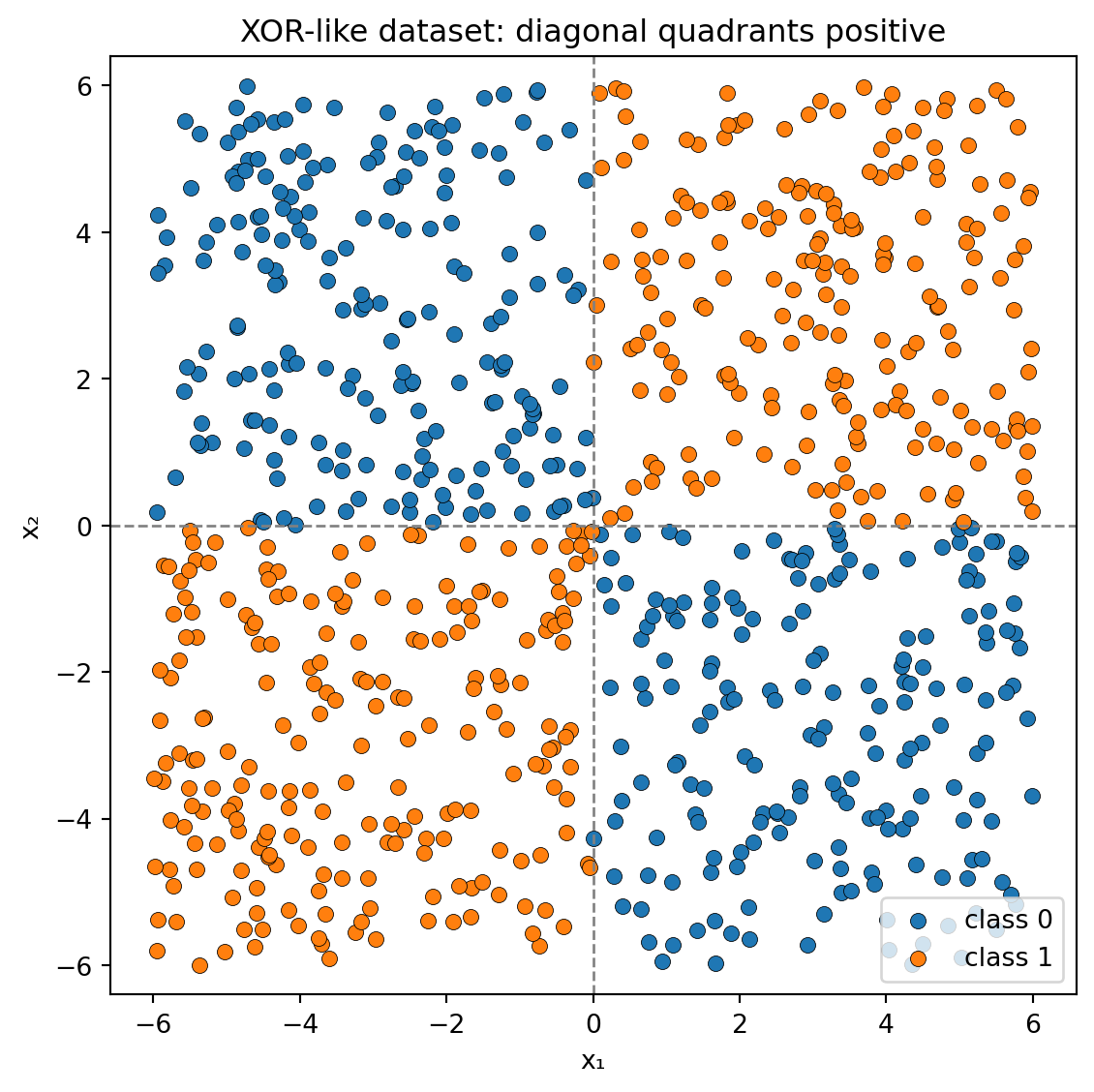
In Lecture 11, a hidden layer was configured by hand to compute Boolean XOR. Here, a continuous version lets us explore learning a nonlinear boundary. Interpret A as (x_1>0) and B as (x_2>0). Class 1 corresponds to A\oplus B: exactly one input is positive, giving the upper-left and lower-right quadrants.
A straight decision boundary cannot separate the classes in the original plane. Both suitable engineered features and a neural network can address this limitation.
The radial feature discards sign information. Points at the same distance from the origin can belong to either class, so the feature that separated the circles cannot separate XOR. In this sampling distribution, the label is independent of the squared radius; a finite sample may nevertheless show small accidental associations.
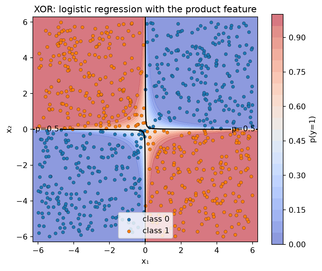
The product s=x_1x_2 distinguishes opposite signs from equal signs. Away from the coordinate axes, class 1 has s<0, while class 0 has s>0. A threshold at zero separates the classes in this feature space.
The quadratic feature expansion already includes x_1x_2. Thus, the full quadratic model can also represent an XOR boundary, even though the radial feature alone cannot.
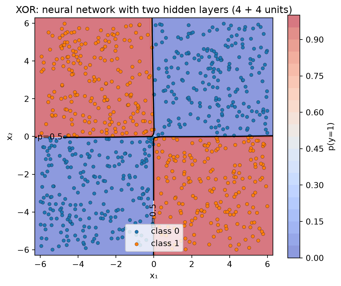
We train a fresh neural network with the same architecture and settings used for the circles. Only the original inputs are provided; we do not supply the radial or product features. The plotting helper and model-building function are reused.
_, xor_test_accuracy = xor_mlp.evaluate(X_test, y_test, verbose=0)xor_scores = {"Logistic: original inputs": xor_raw.score(X_test, y_test),"Logistic: radial feature": xor_radial.score(radial_features(X_test), y_test),"Logistic: product feature": xor_product.score(product_features(X_test), y_test),"Logistic: quadratic features": xor_quad.score(X_test, y_test),"Neural network: original inputs": xor_test_accuracy,}for name, accuracy in xor_scores.items():print(f"{name:<34} test accuracy = {accuracy:.3f}")
Logistic: original inputs          test accuracy = 0.512
Logistic: radial feature           test accuracy = 0.556
Logistic: product feature          test accuracy = 1.000
Logistic: quadratic features       test accuracy = 0.988
Neural network: original inputs    test accuracy = 1.000
Takeaways
Linear separability depends on the representation. A linear classifier on nonlinear features can have a nonlinear boundary in the original input space.
Useful features depend on the task: squared radius separates these circles, while the product distinguishes the XOR quadrants.
Hidden layers provide another way to learn a representation. They do not guarantee that training will find suitable parameters or that a neural network will outperform a model with well-chosen features.
These experiments illustrate Lecture 11’s distinction between what an architecture can represent and what a training process finds from data.